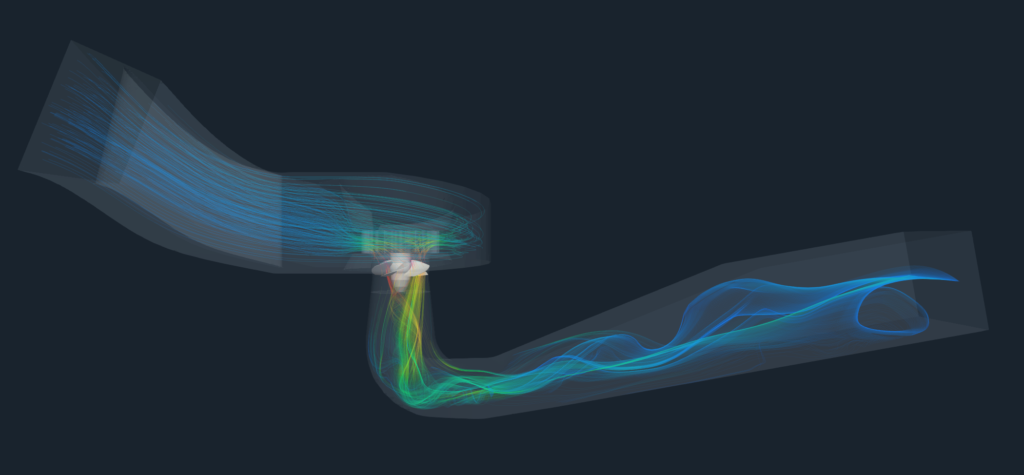
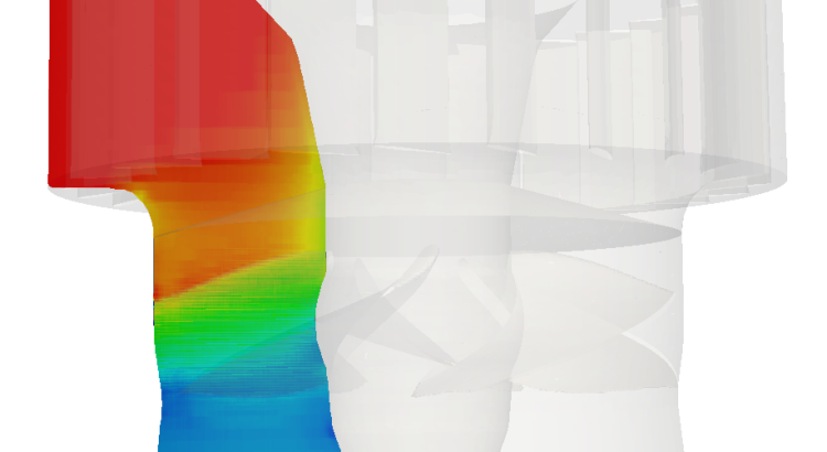
Kaplan Turbine Simulation with TCAE
Understand hydraulic performance, examine structural response, and build a repeatable foundation for better turbine designs.
The engineering objective
Kaplan turbines convert the energy of high-flow, low-head water resources into shaft power. Adjustable runner blades and guide vanes allow their operating characteristics to be matched to changing conditions.
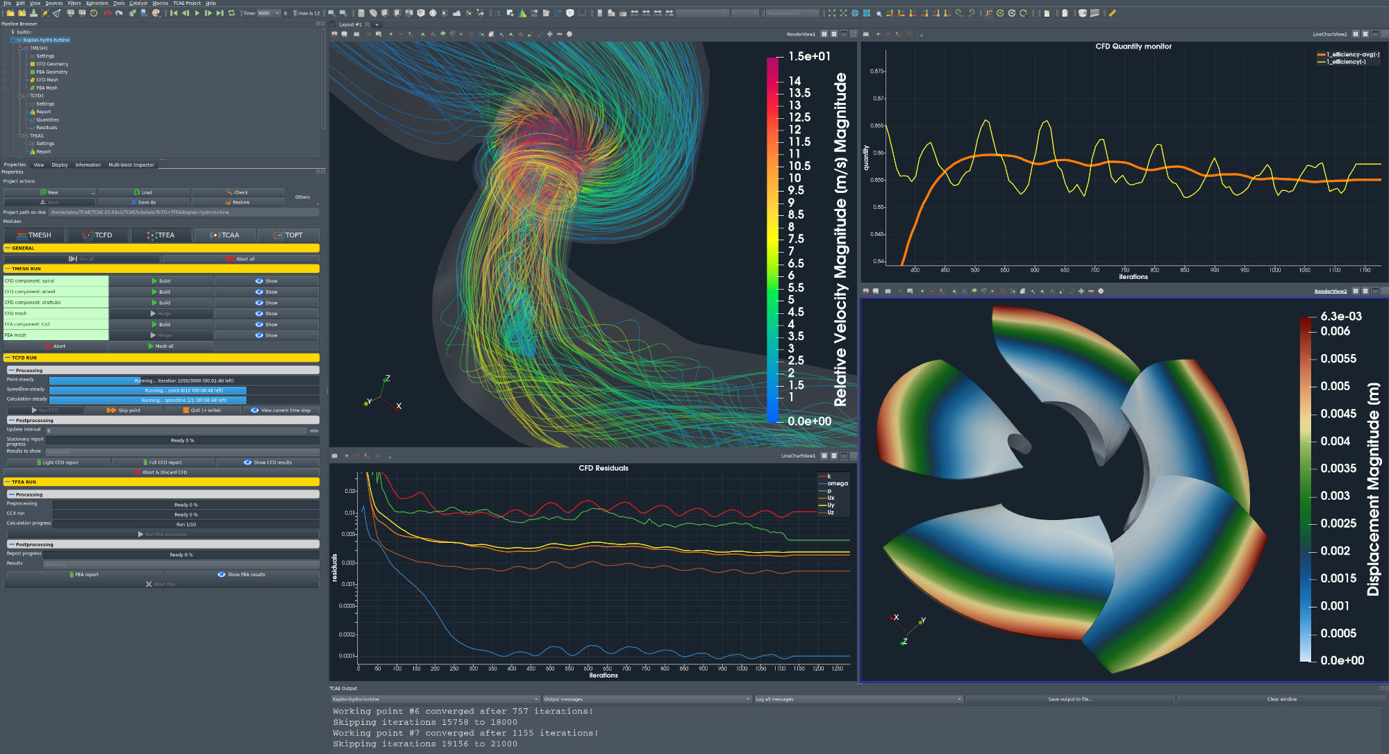
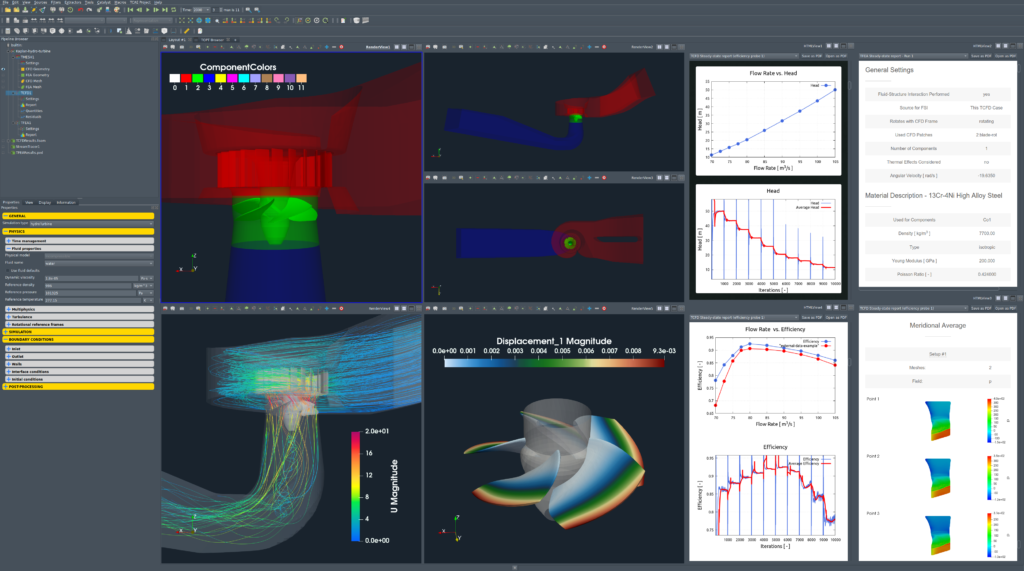
This study examines a Kaplan turbine using TCAE, the CFD SUPPORT simulation environment. It connects geometry preparation, meshing, hydraulic analysis, and reporting in a repeatable workflow. The linked CFD and FEA reports provide the detailed study outputs.
The engineering questions are practical: how does water enter the runner, where are hydraulic losses concentrated, and how do head, torque, and efficiency change with operating point?
The documented baseline is a steady-state, incompressible RANS calculation. It supports assessment of mean flow and performance. Transient pressure fluctuations, rotating vortex ropes, and cavitation require appropriate additional models and studies.
TCAE combines an open-source computational foundation with application-specific workflows and engineering support from CFD SUPPORT. TCFD handles the flow simulation; the wider environment connects meshing, structural analysis, postprocessing, and reporting.
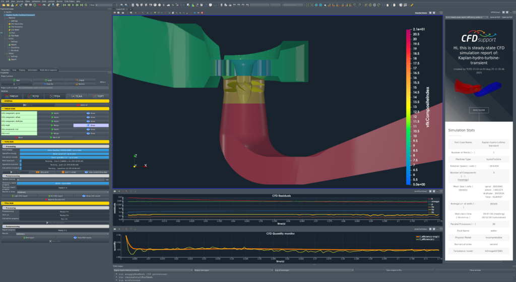
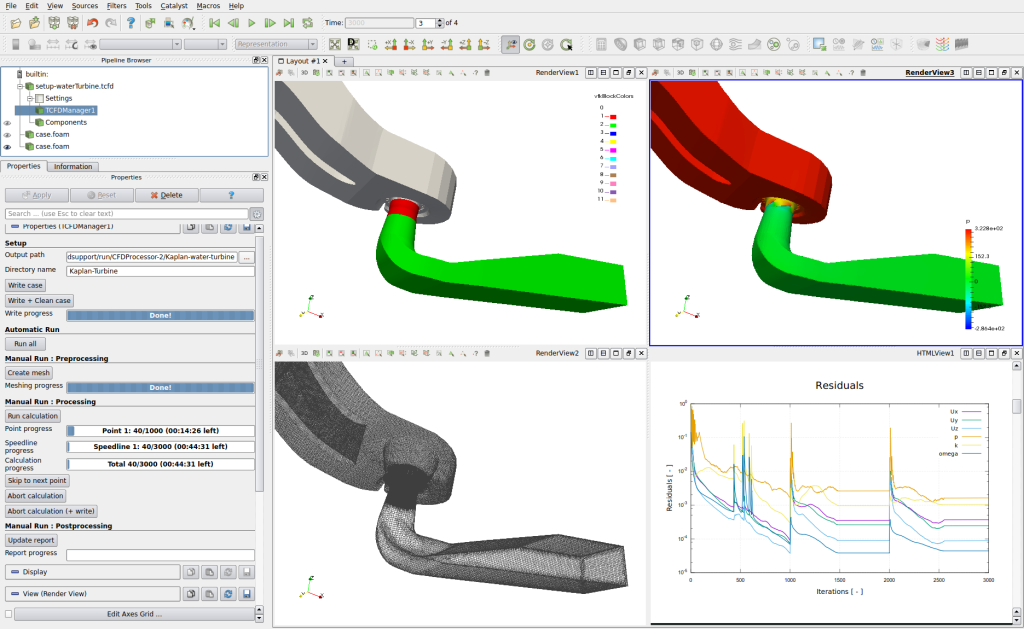
Once the model and settings are defined, the workflow can generate the mesh, prepare and run the calculation, evaluate performance, and produce a report. GUI and batch execution support interactive work and repeated calculations.
This repeatability provides a foundation for agent-assisted work: an agent can coordinate agreed tasks and prepare comparisons while the engineer defines physical assumptions, reviews convergence, and evaluates the evidence.
Geometry and simulation inputs
The starting point is a simulation-ready STL surface model together with operating conditions and fluid properties. External meshes in supported formats, including OpenFOAM and MSH, provide another route.
The domain is divided into connected components, allowing stationary and rotating regions to be meshed separately and coupled through interfaces. Geometry preparation must preserve features relevant to the engineering question, including important clearances and flow passages.
Meshing the flow path
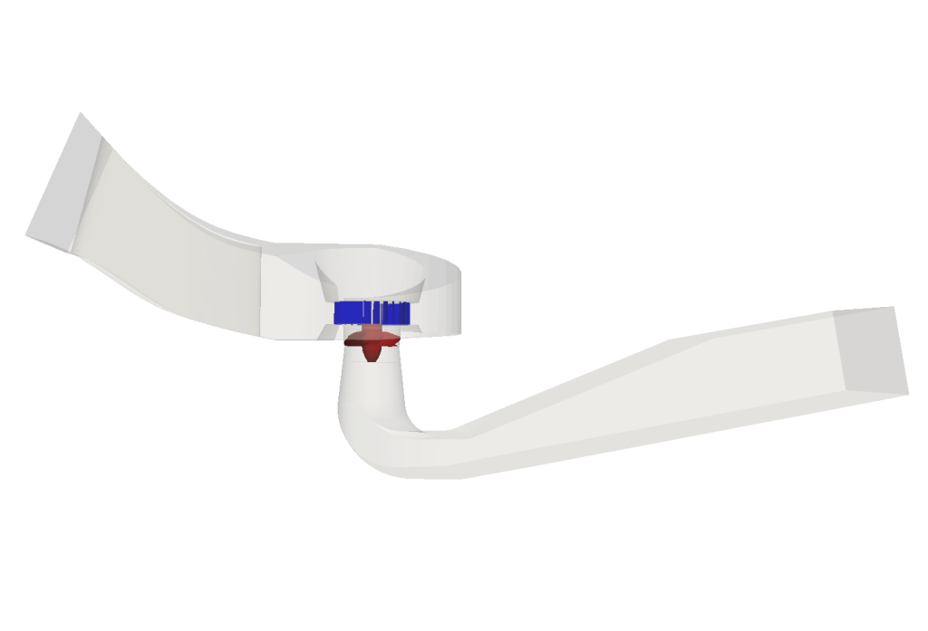
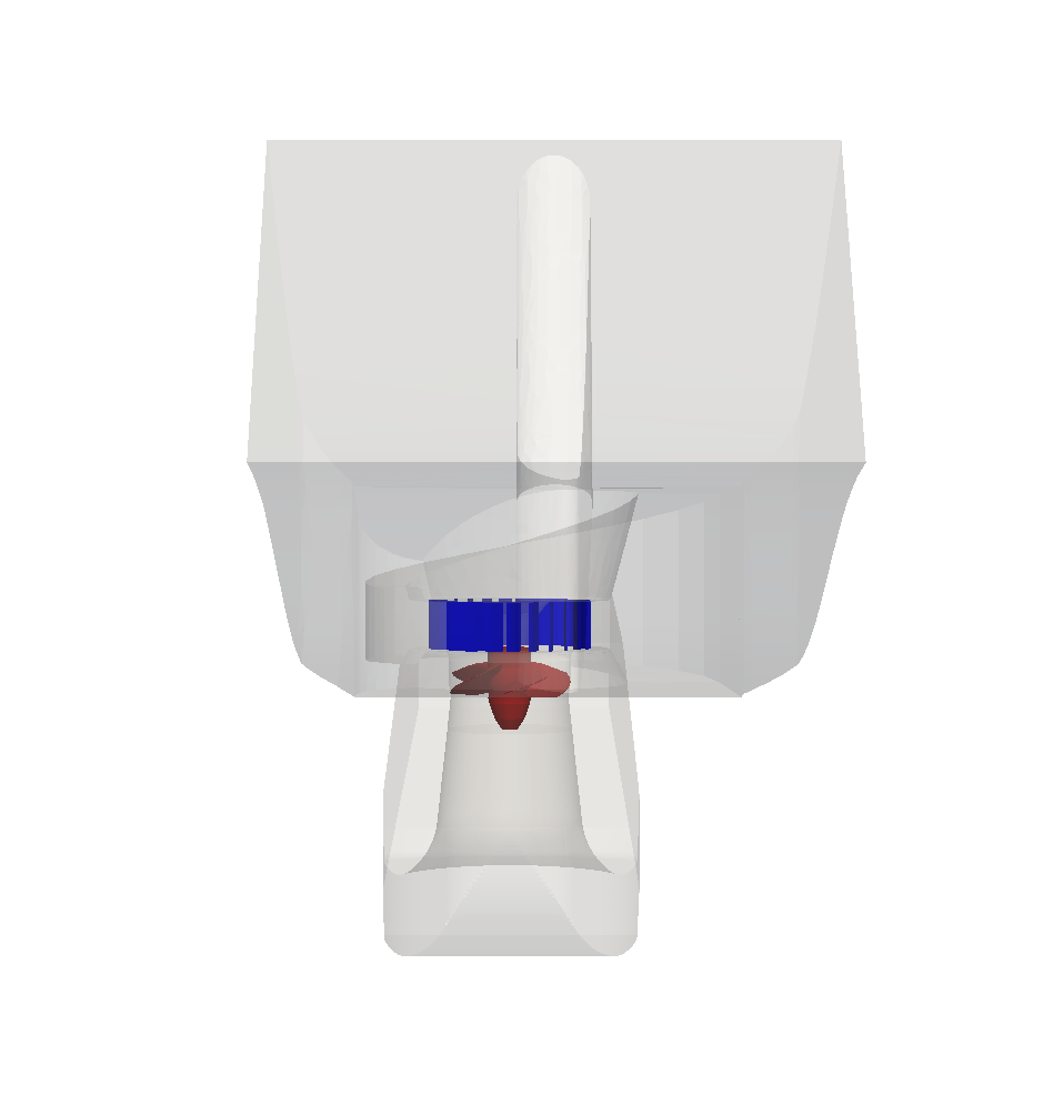
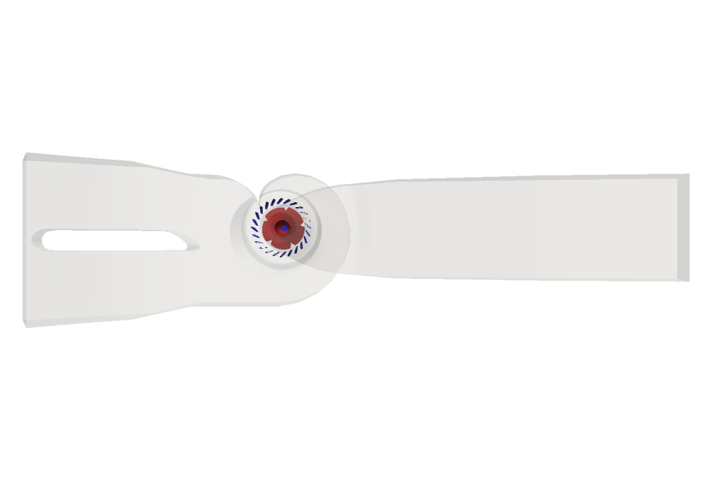
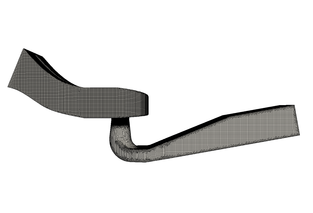
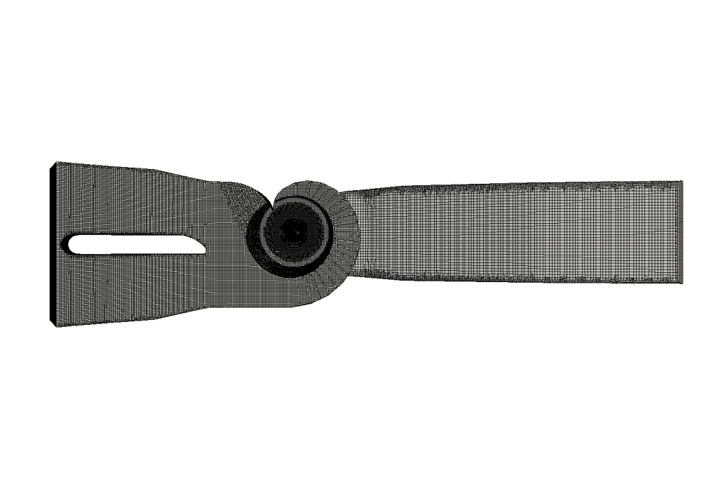
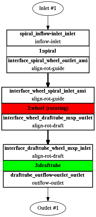
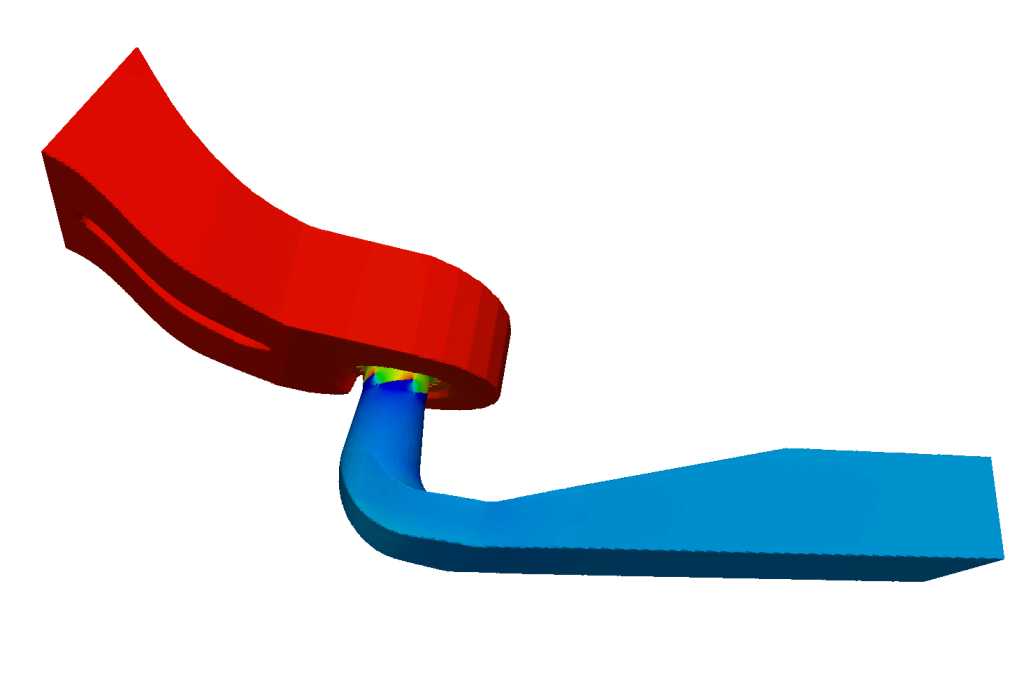
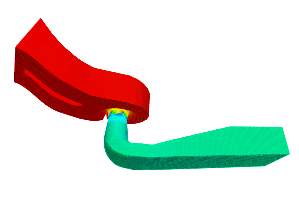
The model has three principal components: the spiral casing, runner, and draft tube. Each component is meshed with snappyHexMesh before the regions are connected for the flow calculation.
The decomposition can be adapted to the study. Separating the casing, stay vanes, guide vanes, runner, and draft tube can help when individual components require different controls or evaluation.
Periodic sector or full runner?
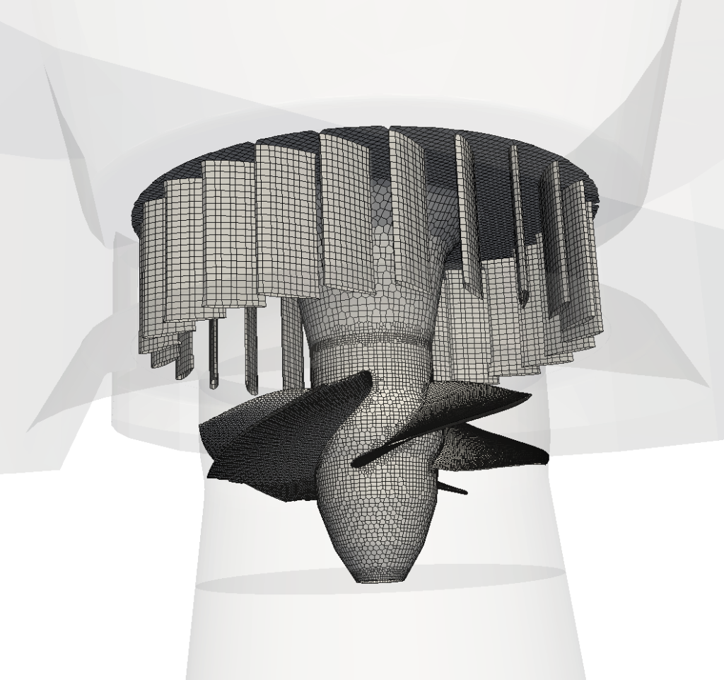
A periodic runner sector reduces the number of cells when geometry, boundary conditions, and interface treatment support the periodic assumption. A full runner retains circumferential variation and provides a basis for studies requiring the complete rotating geometry.
The choice follows the physics to be resolved. A full-runner mesh alone does not make a calculation transient; motion, interfaces, and time-step settings must also be specified.
Near-wall resolution and prism layers
Prism layers near solid walls help control the resolution of velocity gradients. Their design should be consistent with the turbulence model, wall treatment, and local y+ distribution.
The original study reported that omitting these layers could overpredict efficiency by about 1% while reducing CPU cost by roughly 40%. These are case-specific observations, not transferable accuracy or performance guarantees.
Choosing an appropriate mesh resolution
Assess mesh refinement against the quantities that drive the decision: head, torque, efficiency, and relevant local flow features. A change in efficiency with refinement is a sensitivity result, not proof that the finer answer is correct.
Use consistent settings across a sequence of meshes, examine convergence and conservation, and compare with experimental data where available.
Mesh sensitivity: accuracy and computational cost
The original page gives illustrative costs of approximately 4 core-hours per operating point for a coarse mesh without prism layers and 20 core-hours for a finer mesh with layers. Similar integral results can reflect compensating numerical errors; they do not establish mesh independence.
TCAE automation makes systematic comparisons easier to repeat. Record mesh settings, convergence, and performance together, then select a configuration that meets the accuracy requirements of the intended decision.
How the components are connected
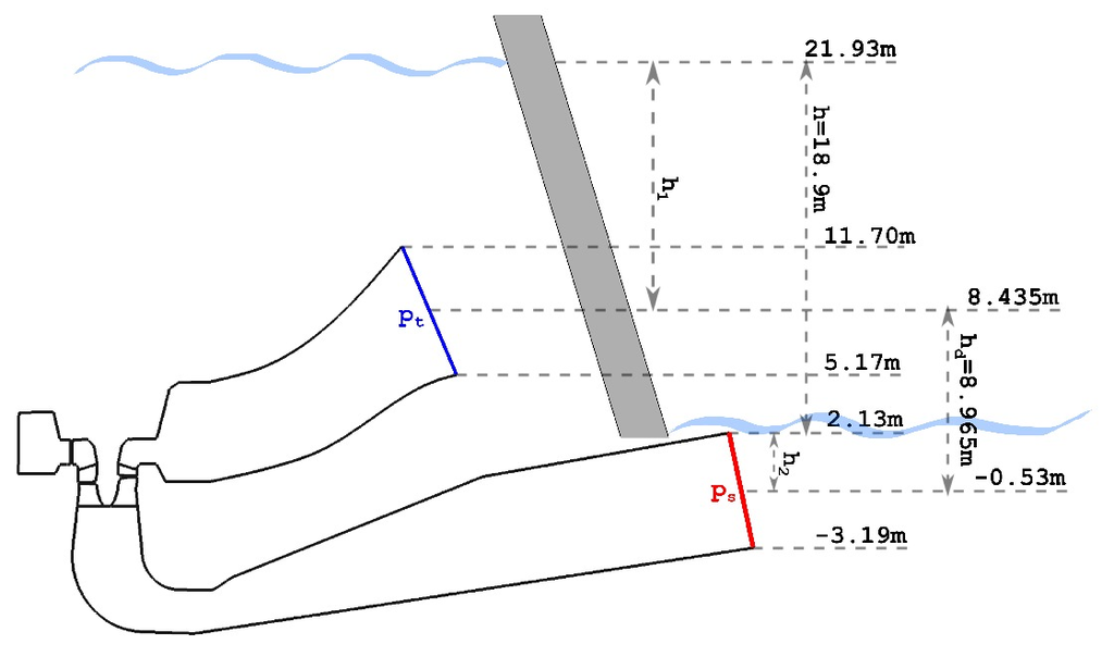
The component graph records the model topology: inlet, outlet, flow regions, and their connections. It provides a compact way to check the flow path before simulation and understand how results relate to each part of the turbine.
Documented CFD setup
- Incompressible flow model
- Steady-state flow model
- Medium: Water
- Viscosity: ν = 8.899e-7 [m2/s]
- Rotation speed: 188 [RPM]
- Flow Rate: 80 [m3/s]
- Interface: mixingInterface (radial averaging)
- Turbulence Model: k-ω SST
- Mesh: snappyHexMesh, hexadominant
- Mesh Cells: 476204
- Mesh Average y+: 155 [-]
- CPU time: 2 [core*hours/point]
Reading the setup: these values describe the historical calculation, not a recommended setup for every Kaplan turbine. Consider the mean y+ of 155 alongside its local distribution and the wall treatment. The listed 2 core-hours per point belongs to this setup; the mesh-comparison examples above describe other configurations.
See the archived TCFD manual for the original reference, and TCAE for current capabilities.
Run, monitor, and compare operating points
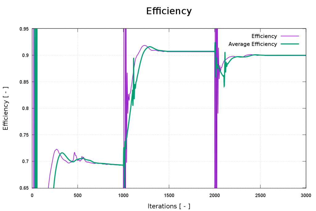
Monitor residuals together with mass balance, torque, head, and efficiency. Accept a calculation against defined convergence criteria, not simply because it has reached a preset iteration count.
Parallel execution can reduce elapsed time, subject to mesh size, hardware, and scaling efficiency. Core-hours describe computational effort rather than wall-clock time.
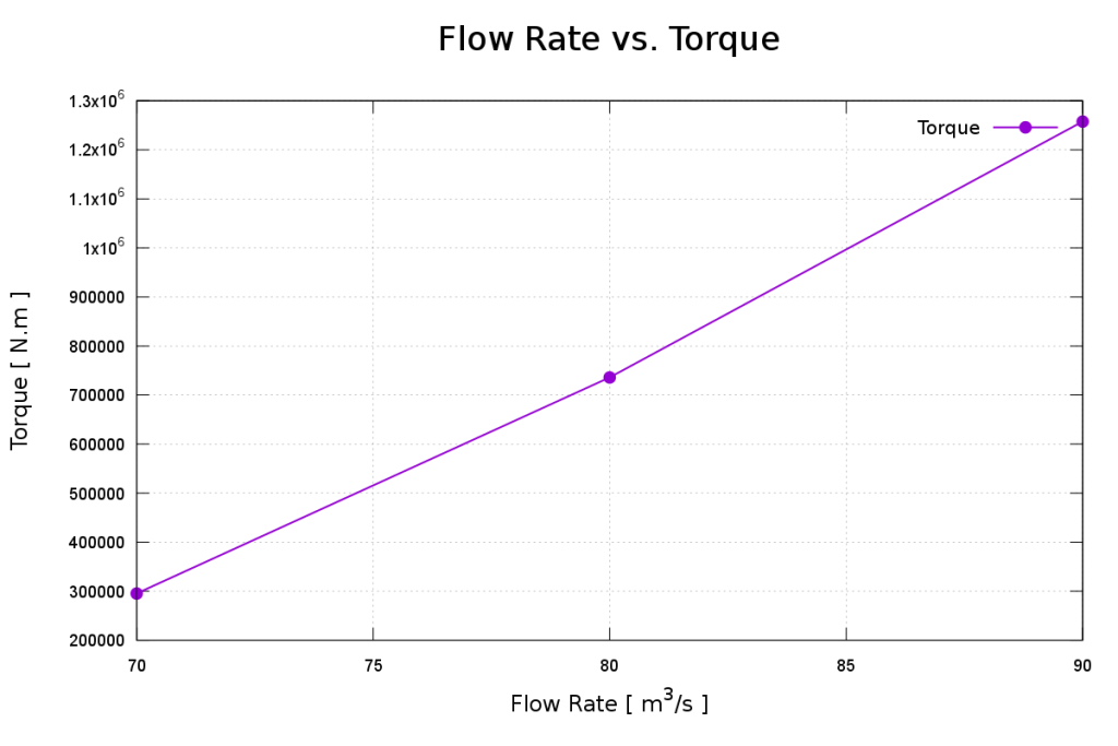
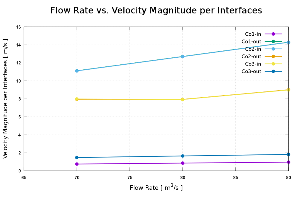
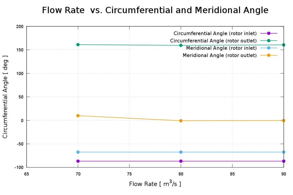
Repeat the workflow across selected operating points to build performance characteristics. Compare converged values consistently and investigate irregular trends before using the curves for design decisions.
Each run produces an HTML report bringing settings, convergence history, and calculated quantities together. Explore the original Kaplan report example alongside the CFD and FEA reports above.
This material illustrates a simulation workflow. It should not be read as an experimental validation claim or evidence of a completed design optimization.
Understand the flow with Turbo Blade Post
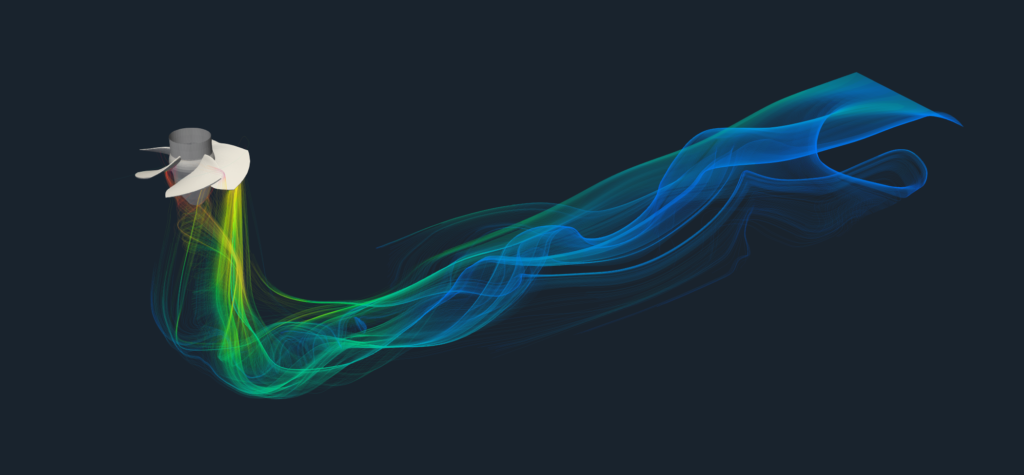
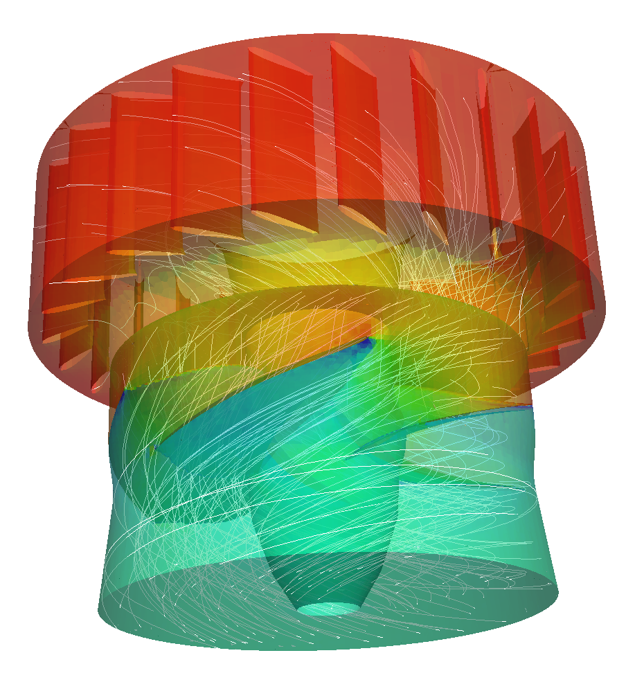
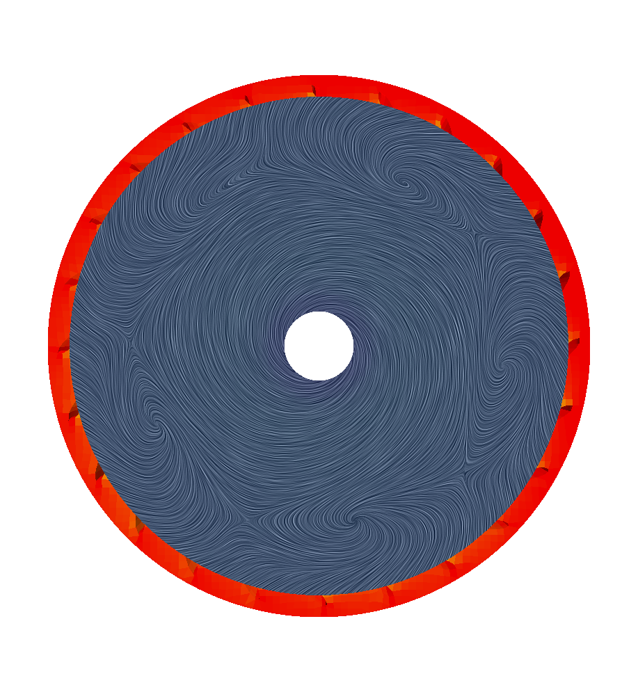
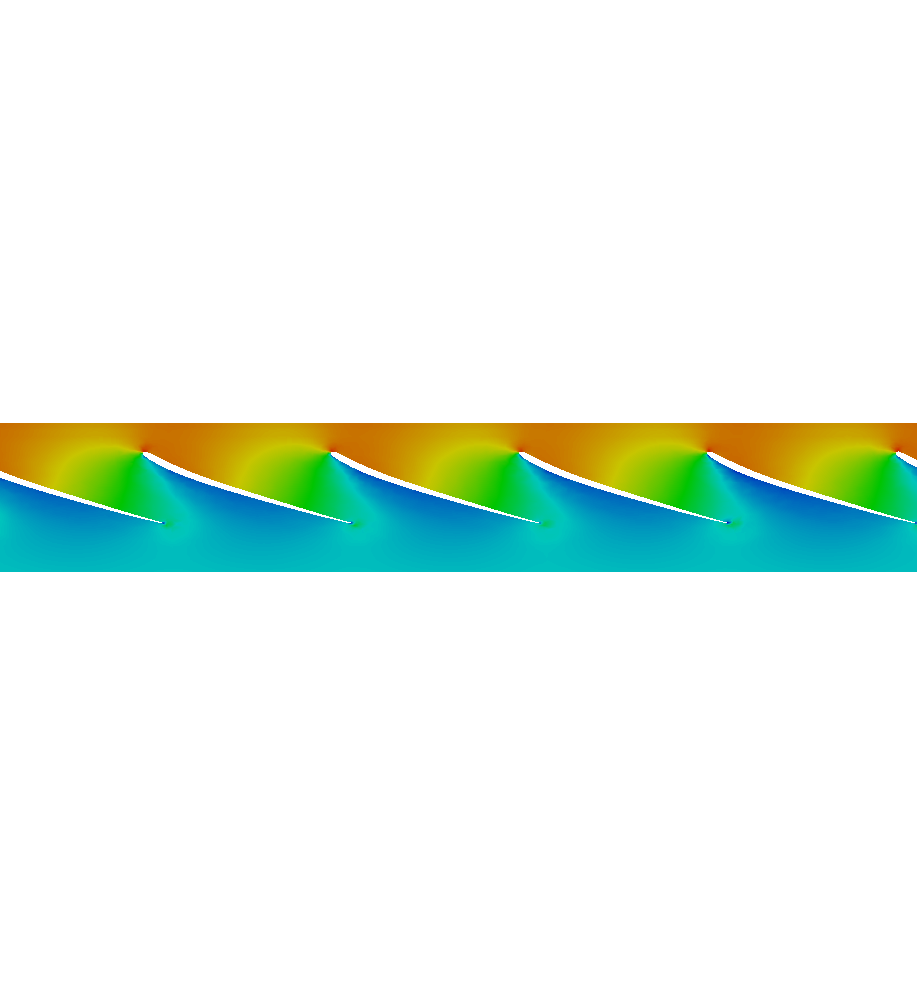
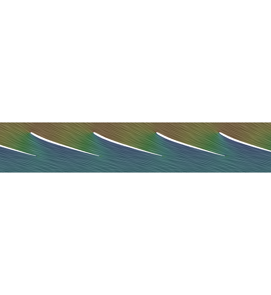
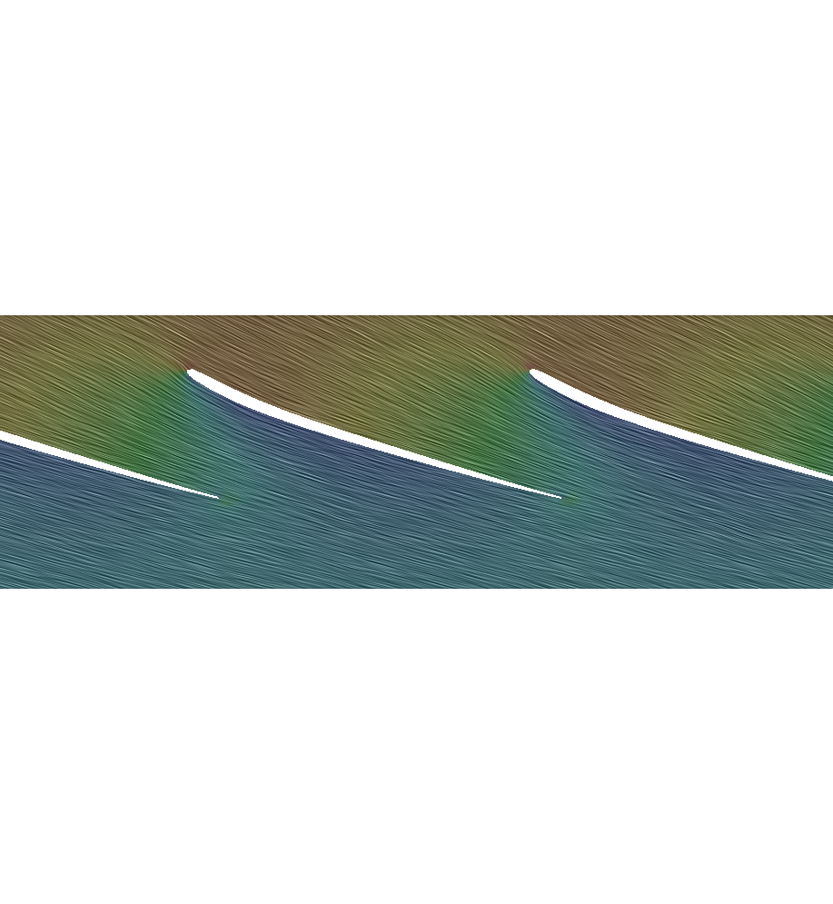
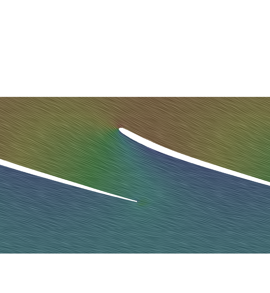
Performance curves show how the turbine behaves; flow-field analysis helps explain why. ParaView provides tools to inspect pressure, velocity, recirculation, and flow entering and leaving the runner.
CFD SUPPORT developed Turbo Blade Post to make turbomachinery results easier to interpret. Blade-to-blade views and meridional averages connect three-dimensional flow features to machine geometry and loading. The online manual explains these operations.
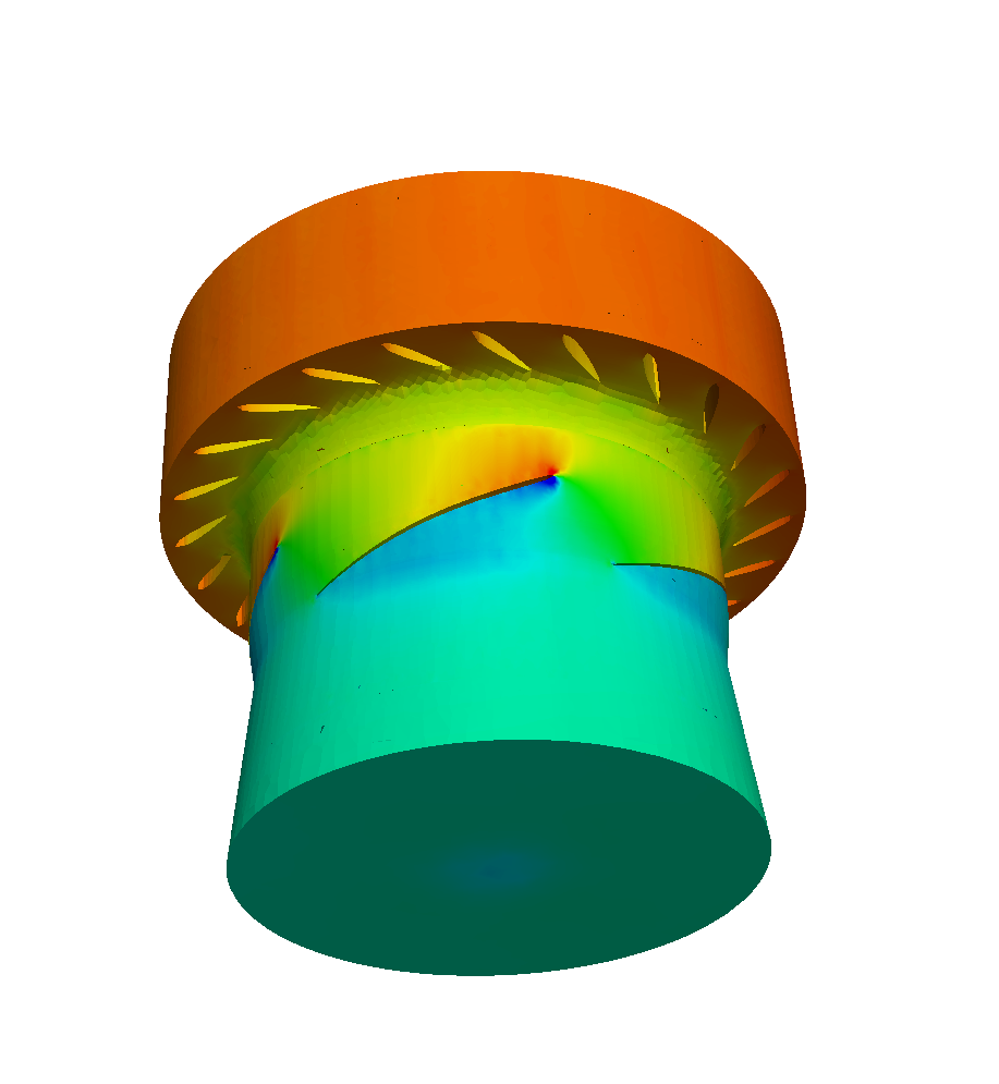
Unwrapping the runner allows results to be examined at a consistent relative span between hub and shroud. These views help compare flow direction, blade loading, and pressure distributions at selected blade heights.
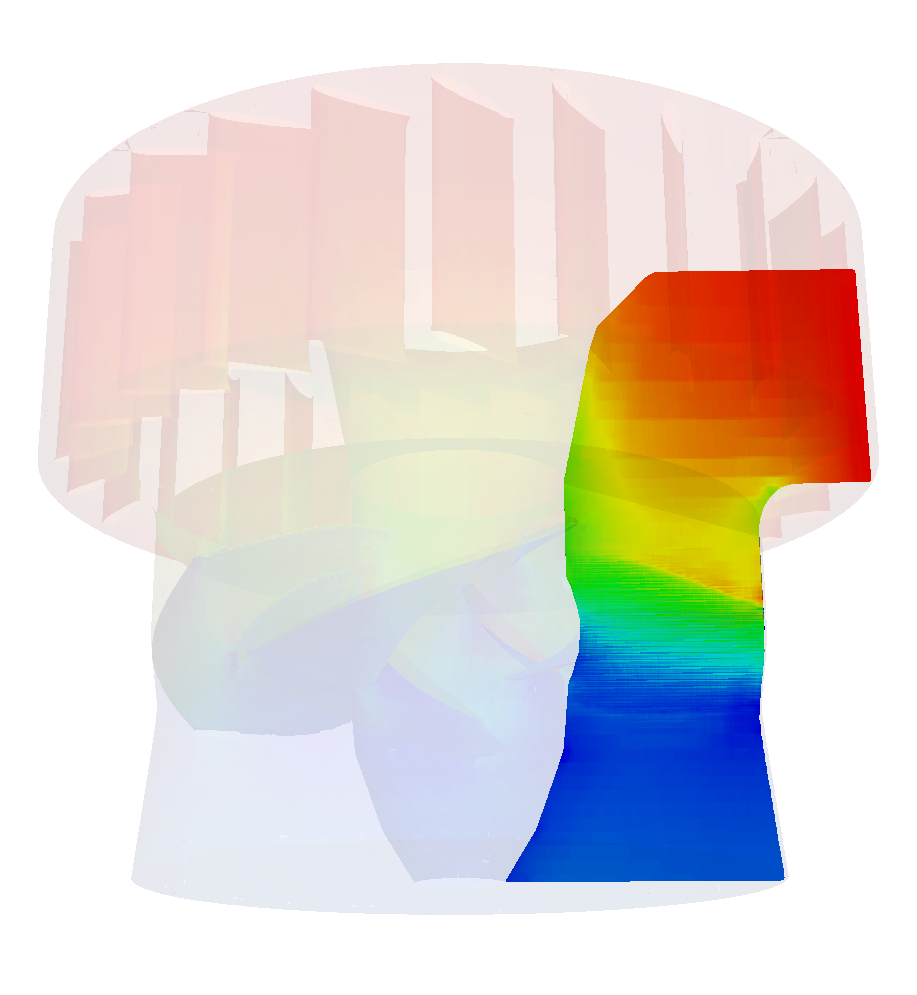
The meridional average projects circumferentially averaged quantities onto the meridian plane, revealing the overall evolution of pressure and velocity through the machine. Use it alongside local views, because averaging can conceal circumferential variations and local extremes.
From a single study to a repeatable design process
This historical Kaplan study is a starting point for a broader workflow: establish a credible baseline, explore alternatives, and retain the evidence for the next project. The following steps describe an extension of the study, not additional results from the original calculation.
Coordinate the work with an agent
The engineer defines the operating envelope, assumptions, and evaluation criteria. An agent can help prepare cases, execute the agreed TCAE workflow, track runs, and assemble comparisons. Failed runs and changes to the physical model should remain traceable. The engineer reviews the evidence and makes the decision.
Explore alternatives with TOPT
TOPT extends repeated simulations into parametric studies and optimization. For a suitably parameterized Kaplan model, variables could include runner pitch, guide-vane opening, or geometric parameters. Objectives could consider efficiency across several operating points, subject to hydraulic and structural constraints. Proposed improvements still need verification with an appropriate simulation methodology.
Retain engineering knowledge with TBASE
TBASE provides the knowledge-management direction: retain design parameters, operating conditions, model settings, and results together. Consistent datasets support later comparisons and, where suitable models are available and validated, surrogate-assisted exploration. Predictions need checks within their supported range, and promising designs need simulation verification.
Engineers define the objectives. Agents coordinate the work. TCAE executes the simulation workflow. TOPT explores alternatives. TBASE helps retain and reuse the knowledge.
Apply the workflow to your turbine
CFD SUPPORT can help you define the modelling approach, establish a repeatable workflow, and interpret the results. Whether you want to run TCAE independently or develop an agent-assisted process, the starting point is your engineering question.
Download the Kaplan turbine tutorial
File name: Kaplan-hydro-turbine-TCAE-Tutorial.zip
File size: 7 MB
Tutorial focus: Kaplan hydro turbine; water flow; three-component model; automated meshing; steady-state CFD; performance evaluation; CFD and FEA reports; turbomachinery postprocessing.