Mechanical Siren Acoustic Tutorial
This case study shows a complex CFD + CAA workflow of Mechanical Siren using simulation environment TCAE
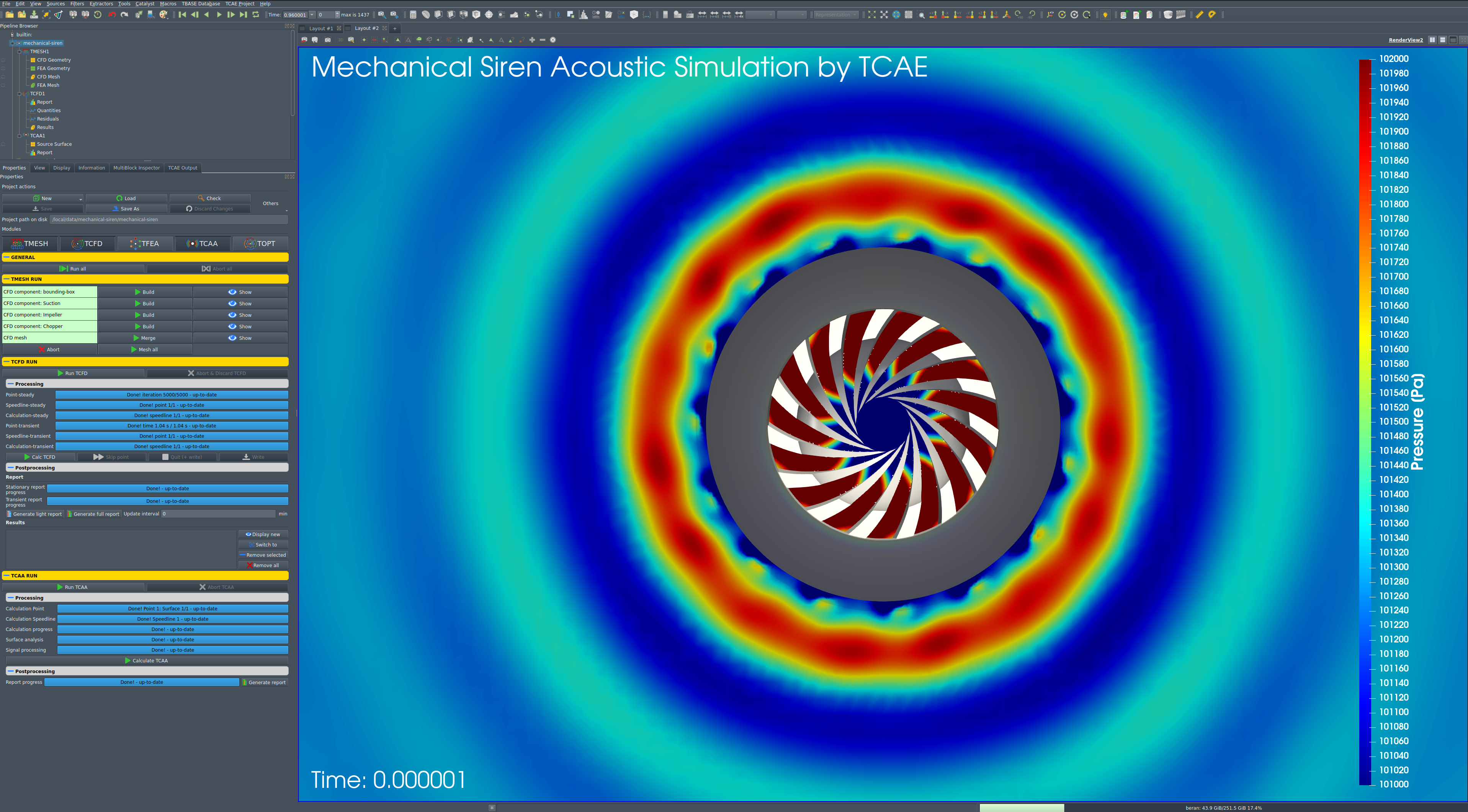
In this project, we deal with the engineering simulation workflow of Computational Aero-Acoustics (CAA). This study deals primarily with CFD simulation and the evaluation of the acoustic properties from the pressure. The whole simulation process is demonstrated in the TCAE simulation environment.
Employing advanced techniques like resolved CFD simulation together with the Acoustic Analogy and Ffowcs Williams-Hawkings, we explore the transient simulation with Finite Volume CFD simulations in a cell-centered framework. The mesh generation utilizes SnappyHexMesh with inflation layers powered by OpenFOAM and within the TCAE environment. Our study employs the k ω SST-DES model. We assess the Sound Pressure Level (SPL), Power Spectral Density (PSD), present Polar plots, and backward sound reconstruction. This comprehensive analysis sheds light on the fascinating world of CAA and its applications in aerodynamics.
Mechanical Siren Acoustic Tutorial - Input Data
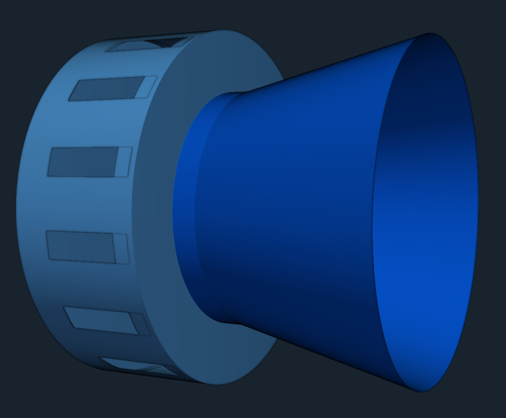
The input data for this case study is the CAD model (the digital representation of the real device) which has been for simulation purposes processed in the Salome open-source software. Any other standard CAD system can be used instead.

Mechanical Siren Acoustic Tutorial - CFD Simulation Preprocessing
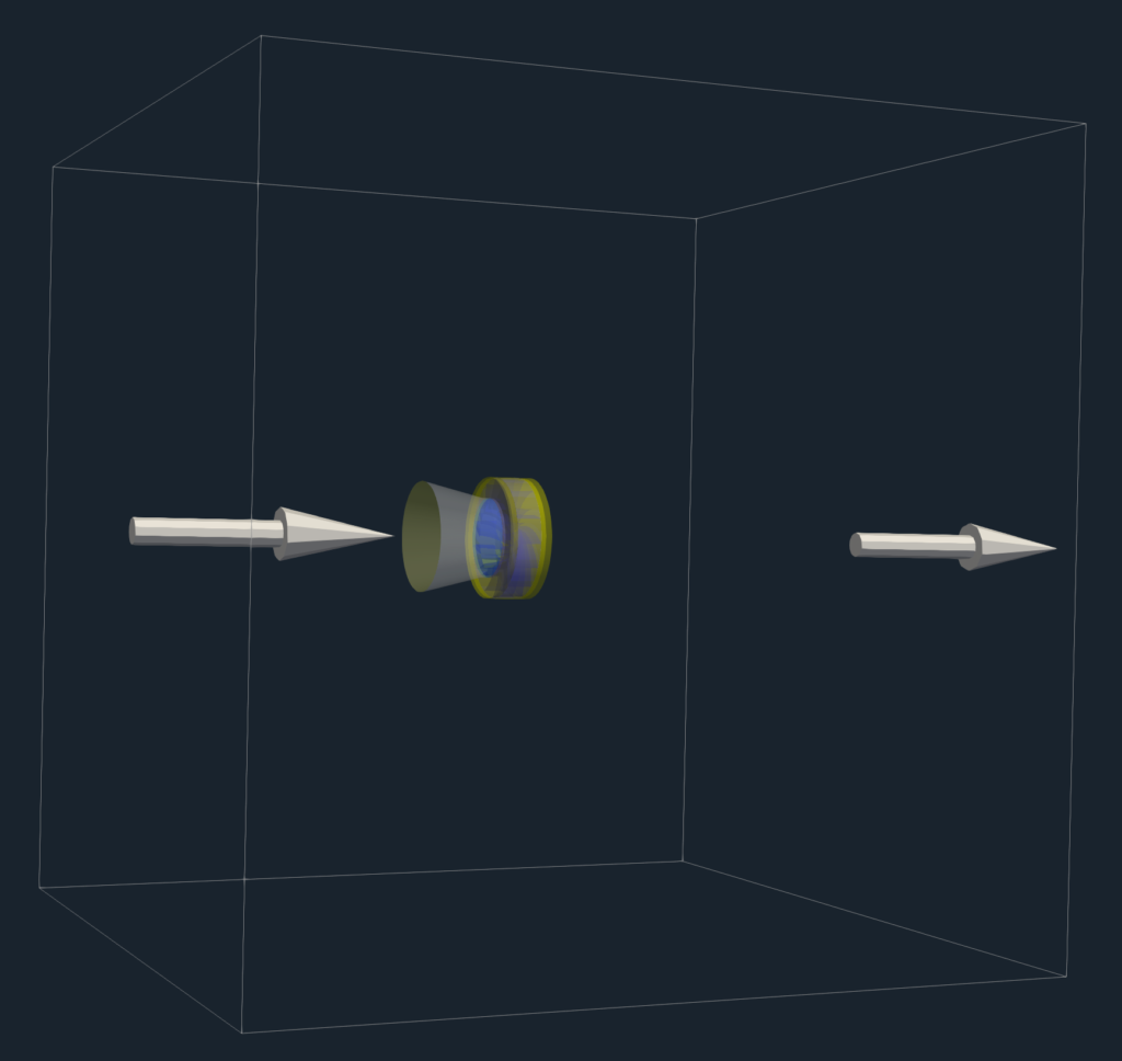
A typical input for a detailed simulation analysis is a 3D surface model in the form of an STL surface, together with related physics and boundary conditions. For CFD simulation, it is needed to have a simulation-ready surface, which is a closed watertight model (sometimes also called waterproof, model negative, or wet surface) of the model’s parts where the fluid flows. The simulation domain consists of two chambers divided by a wall. The mechanical siren is closed in a virtual domain.
For CFD simulation it is best to split the geometry into several waterproof components because of rotation (some parts may be rotating and others not). Each component itself has to be waterproof and consists of a few or multiple STL surfaces. It is smart to split each component into multiple surfaces (more is better) because it opens a broader range of meshing options, simulation methods (mesh refinements, manipulation, boundary conditions, evaluation of results on model-specific parts, …), and postprocessing.
This CAD model is relatively simple. The final surface model in the STL format is created as input for the meshing phase. This preprocessing phase of the workflow is extremely important because it determines the simulation potential and limits the CFD results.
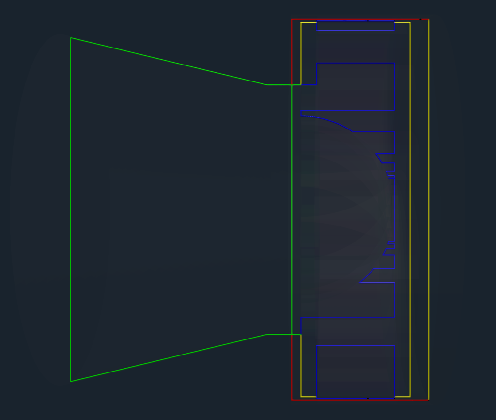
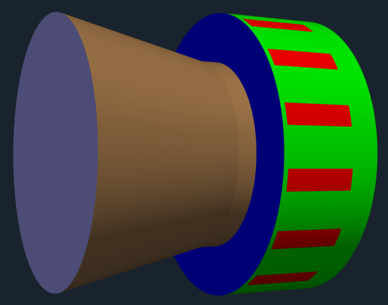
In this project, the model has been split into four logical parts:
- External virtual domain – Bounding Box
- Suction
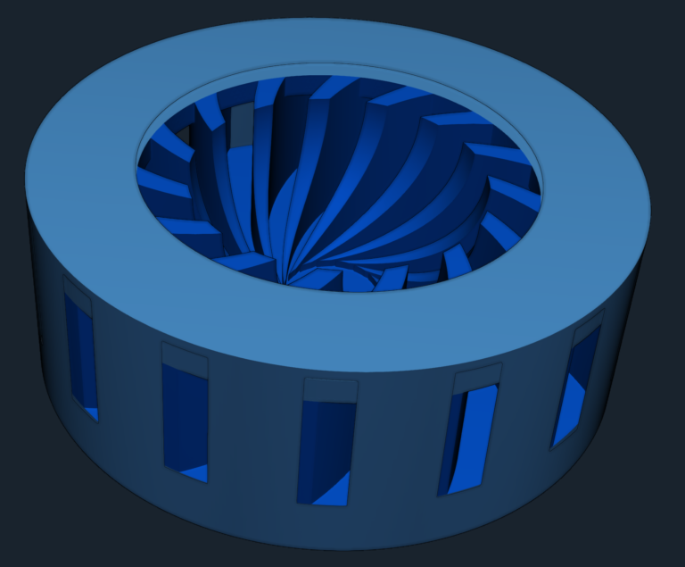
- Impeller
- Chopper
In the CFD methodology employed for this study, the surface model data, representing the geometry, is stored in .stl file format. Along with the geometric information, the necessary physical inputs, such as boundary conditions and material properties, are also loaded into the TCFD software.
In addition to the .stl file format, there are alternative options available for mesh loading in TCFD. Users have the flexibility to import an external mesh in OpenFOAM mesh format, which offers compatibility with other simulation tools within the OpenFOAM framework. Alternatively, TCFD supports loading meshes in MSH format (Fluent mesh format) or CGNS mesh format, providing a wider range of mesh compatibility options.
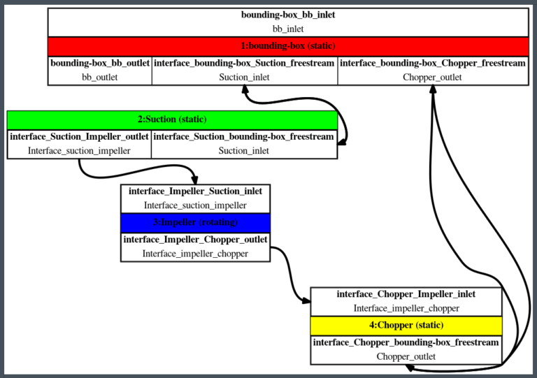
TCFD module follows a multi-component approach. This means that the model is divided into several distinct components or regions, each serving a specific purpose or containing specific properties. In TCFD, each region can have its own dedicated mesh, allowing for finer control over the discretization and resolution of different regions within the model.
This CFD methodology employs a multi-component approach, which means the model is split into a certain number of components. In TCFD each region can have its own mesh and individual meshes communicate via interfaces.
IMPORTANT NOTICE ON PREPROCESSING
The surface of the simulation-ready model has to be clean, simple enough but not simpler! The principles are always the same: the watertight surface model has to be created; all the tiny, irrelevant, and problematic model parts must be removed, and all the holes must be sealed up (the watertight surface model is required). The preprocessing phase is an extremely important part of each simulation workflow. It sets up all the simulation potential and limitations. It should never be underestimated. Mistakes or poor quality engineering in the preprocessing phase can be hardly compensated later in the simulation phase and postprocessing phase. For more details, see the TCAE documentation.
CFD Mesh Setup
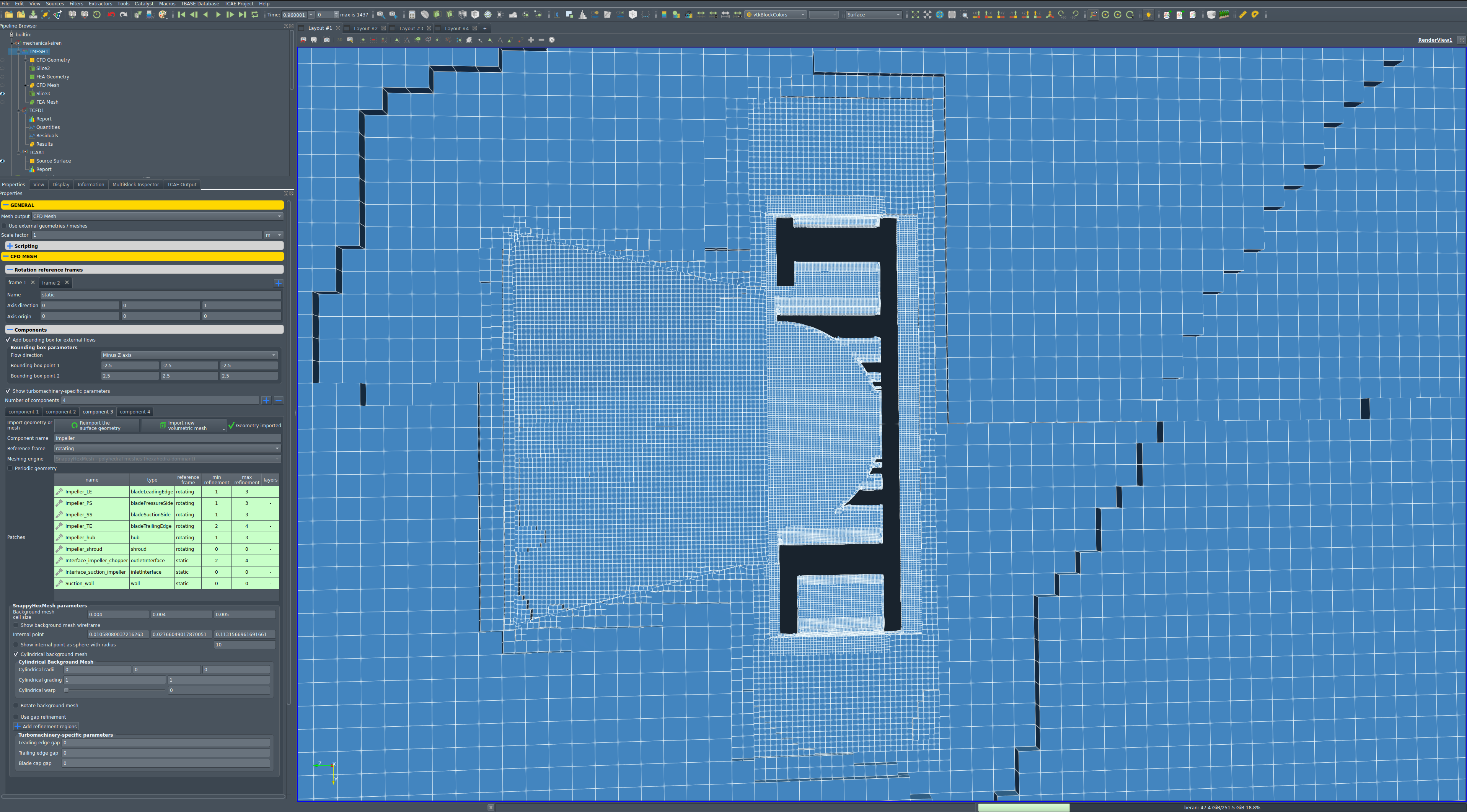
Baseline mesh statistics
- Hexahedra-dominant mesh
- snappyHexMesh
- Domain size: 2.5 x 2.5 x 2.5 [m]
- Number of components: 4 [-]
- Basic cell size in the impeller component: 4 [mm]
- Cells' sizes close to the blade: < 0.1 [mm]
- Number of inflation layers: 0 [-]
- Final mesh cell count: 4 904 007 [cells]
- Y+ min: 0.05 [-]
- Y+ max: 85.6 [-]
Mechanical Siren - CFD Simulation Setup
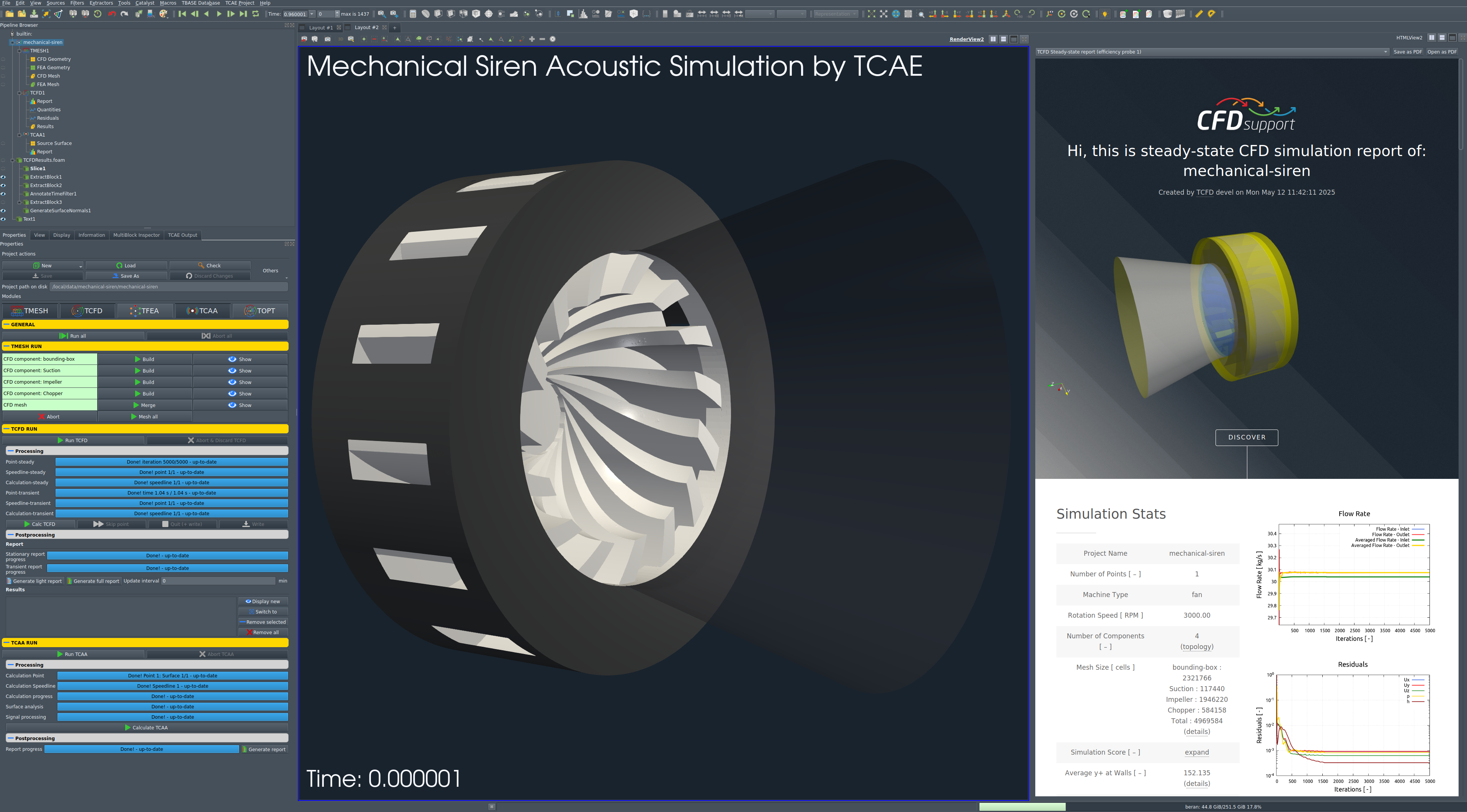
The CFD simulation in this project is facilitated through the utilization of the TCAE software module TCFD. The entire setup and execution of the CFD simulation are performed within the TCFD GUI integrated with ParaView. TCFD, being based on the OpenFOAM open-source software, provides a powerful foundation for accurate computational fluid dynamics simulations.
The simulation setup process involves navigating through the GUI from the top menu to the bottom, allowing for a systematic configuration of various parameters and settings. This GUI-driven approach ensures a user-friendly experience and enables researchers to define the simulation environment in a step-by-step manner, tailoring it to the specific requirements of the study. By leveraging the intuitive interface, researchers can efficiently set up their simulation, defining boundary conditions, solver options, mesh properties, and other relevant aspects, leading to a comprehensive and accurate CFD simulation.
- Simulation type: Fan
- Time management: Transient - 50 revolutions
- Physical model: Compressible
- Number of components: 4 [-]
- Wall roughness: none
- Speed: 3000 [RPM]
- Outlet: Static pressure 0 [m2/s2]
- Turbulence: DES-SST
- Temperature: 293.15 K
- Viscosity model: Newtonian
- Wall treatment: Wall functions
- Turbulence intensity: 5%
- Speedlines: 1 [-]
- Simulation points: 1 [-]
- Fluid: Air
- Reference pressure: 1 [atm]
- Dynamic viscosity: 1.8 × 10E-5 [Pa⋅s]
- Reference density: 1.2 [kg/m3]
- CFD CPU Time: 2500 core.hours
- BladeToBlade: off
TCAA Setup
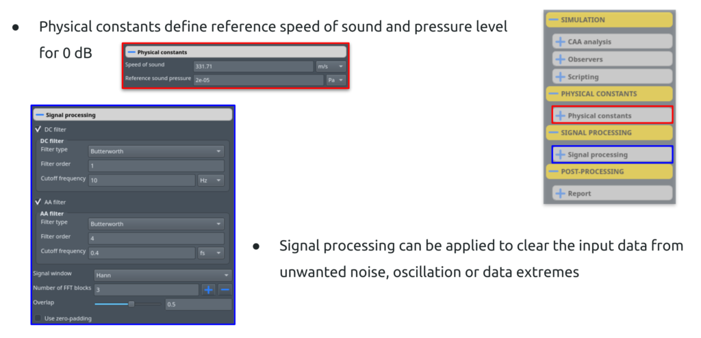
Acoustic Signal Processing
While the CFD simulation is completely run in the TCFD module. All the acoustics-related settings and later evaluation are done in the TCAA module. A few notes on the signal processing setup:
- The raw signal is centered on the origin and Butterworth filters are applied
- The Welch method is used to transfer the signal to the frequency spectrum
- The signal is divided into three overlapping segments
- On each segment, the Hann window is applied and the Fourier transform is executed
- Transformed segments are reassembled
- PSD and SPL are evaluated from the final signal in the frequency domain
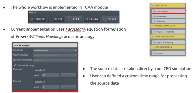
- The current implementation uses the Farassat1A equation formulation of Ffowcs-Williams Hawkings acoustic analogy
- The source data are taken directly from the CFD simulation
- Users can define a custom time range for processing the source data
- Observer is a point in the far field where the acoustic pressure is evaluated by acoustic analogy
- The observer’s location can be also imported from the file to define a more general distribution
- Physical constants define the reference speed of sound and pressure level for 0 dB
- Signal processing can be applied to clear the input data from unwanted noise, oscillation, or data extremes
Observers
The far-field approach is a method used to study the propagation and characteristics of sound waves generated by aerodynamic sources (fan blades). The acoustic signal is evaluated in predefined locations – observers. Observers are virtual points typically located in positions of microphones to allow the direct comparison of the simulation results and physical measurements.
Three observer groups are used. First observer is located 60 cm away from the center along the x-axis. The second observer is located 6 m away from the center along the x-axis. The third is group of 50 observers distributed symmetrically along the siren in distance 3 m.
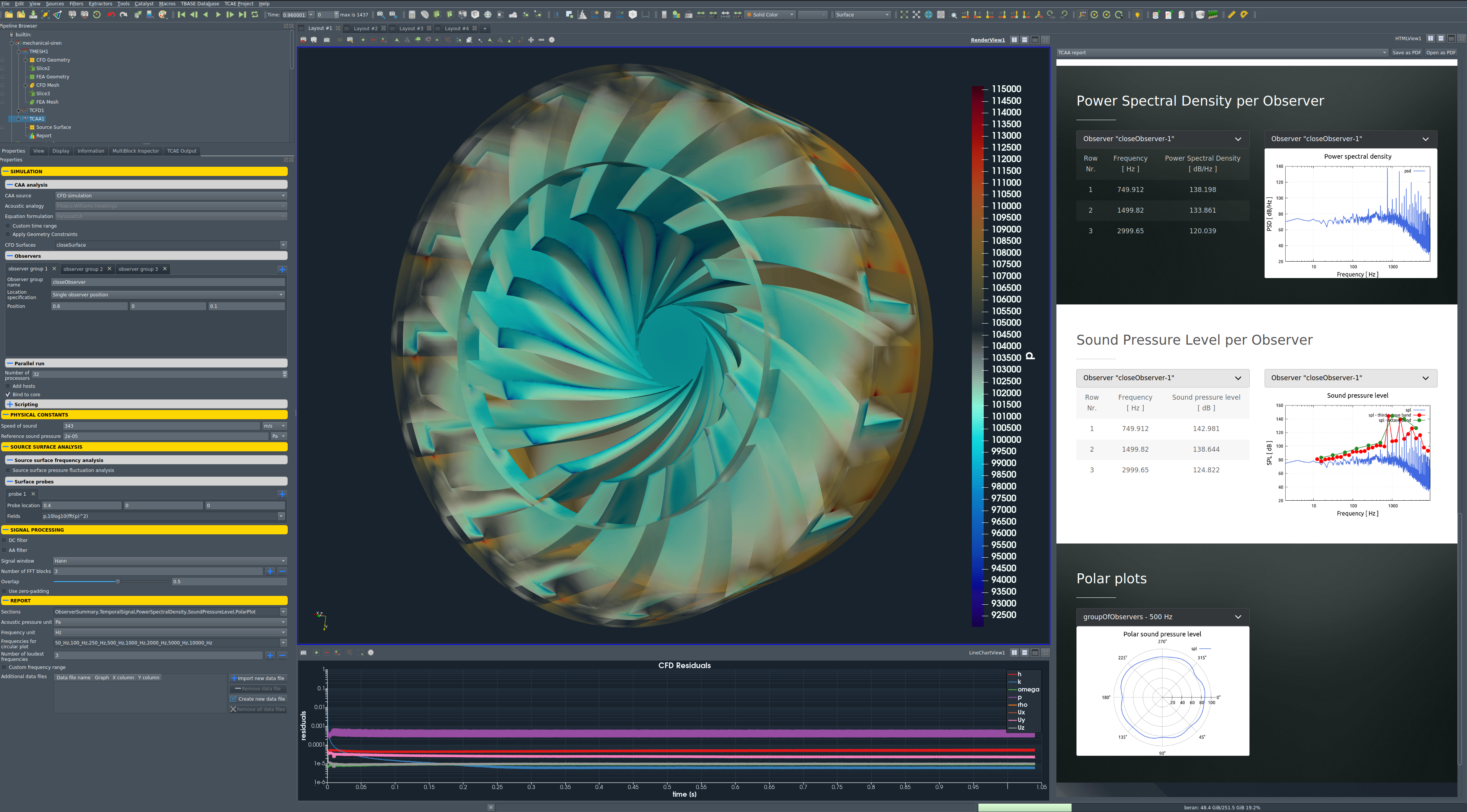
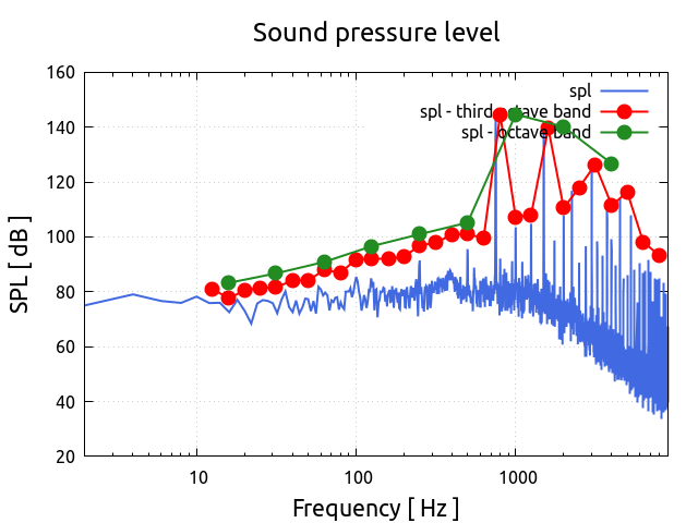
Sound Pressure Level - SPL - Evaluation
One of the main results of the acoustic simulation is the Sound Pressure Level – SPL.
Sound pressure or acoustic pressure refers to the deviation in pressure from the average or equilibrium atmospheric pressure, induced by the presence of a sound wave. This deviation in pressure propagates through a medium, such as air or water, as the sound wave travels, transmitting the auditory information perceived by humans and other organisms. Sound pressure serves as a fundamental metric in the study of acoustics, allowing researchers to quantify the intensity and characteristics of sound waves in various environments and scenarios.
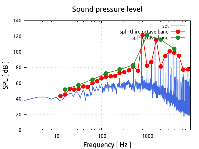
The third-octave band of the Sound Pressure Level (SPL) refers to a graphical representation that breaks down the SPL into its frequency components across different frequency bands. In this representation, the frequency range of interest is divided into octave bands, and each octave band is further subdivided into three equal parts, known as third-octave bands.
Each third-octave band corresponds to a specific range of frequencies, and the SPL within each band is measured or calculated. By analyzing the SPL across these frequency bands, engineers and researchers can gain insights into the frequency distribution of sound energy in a particular environment or from a specific source. This information is valuable for various applications, including noise control, environmental noise assessment, and acoustic design.
Observer #1
Observer #2
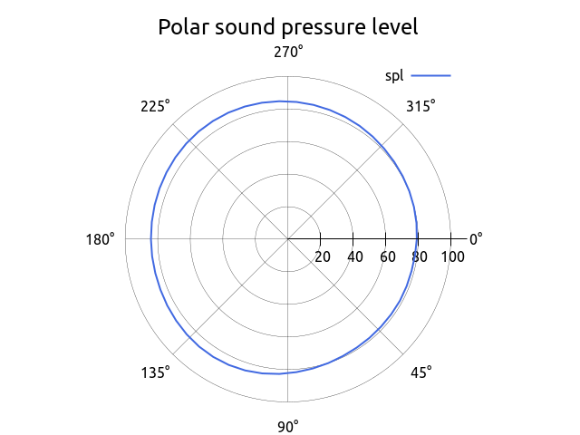
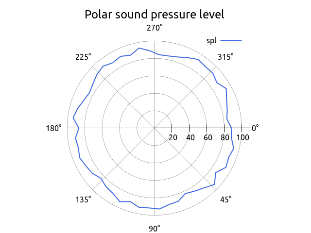
Sound Pressure Level - Polar Plots
Sound Pressure Level (SPL) Polar Plots provide a visual representation of the distribution of sound pressure levels across different directions in a given space. Each point represents an individual observer placed on the circle around the object.
In these plots, the radial distance (circle, R = 1m) from the fan center (Two circles: 1. circle around the horizontal (rotational) axis, 2. circle around the vertical axis) represents the distance from the sound source, while the angular direction (angle) indicates the direction of measurement. Each point (90 points by 4 degrees) on the plot corresponds to a specific angle and distance from the source.
These plots are particularly useful for analyzing the directional characteristics of sound fields, such as those generated by acoustic sources. By examining the SPL distribution across various angles, engineers and researchers can gain insights into how sound propagates in different directions from the source, aiding in the design of sound control measures, acoustic treatments, or optimization of noise-reducing devices.
Selected Polar Plots
250 Hz
500 Hz

1000 Hz
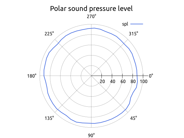
2000 Hz
Power Spectral Density - PSD - Evaluation
Power Spectral Density (PSD) represents the distribution of power into frequency components composing that signal. It describes how the power of a signal or time series is distributed with frequency.
Observer #1
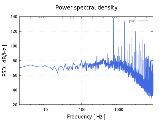
Observer #2

TCAA Sound Reconstruction
TCAA can reverse the procedure and reconstruct the sound out of the simulation results.
Observer #1
Observer #2
Conclusion
- It has been shown how to make a comprehensive Computational Aero-Acoustics analysis on a Mechanical Siren in a single automated workflow.
- There was no special tuning used in the CFD simulation at all. There remains a lot of space for tuning CFD methodology, especially for mesh resolution, turbulence modeling, and numerical schemes.
- TCAE has shown to be a very effective tool for Computational Aero-Acoustics simulations
- This benchmark was intentionally written so short not to overwhelm its reader with too many details. The original intention was to show the modern simulation workflow and its accuracy.
- The benchmark details are listed in the references below.
- All the technical details regarding CFD & FEA simulation are listed in the TCAE Manual.
- The benchmark geometry and data are freely available for download on the CFDSUPPORT website https://www.cfdsupport.com.
- More information about TCAE can be found on CFD SUPPORT website: https://www.cfdsupport.com/tcae.html
- Questions will be happily answered via email info@cfdsupport.com.
References
Download TCAE Tutorial - Mechanical Siren Acoustic Tutorial
File name: mechanical-siren-TCAE-Tutorial.zip
File size: 133 MB
Tutorial Features: CFD, CAA, TMESH, TCFD, TCAA, SIMULATION, COMPRESSIBLE FLOW, TRANSIENT FLOW, AUTOMATION, WORKFLOW, SNAPPYHEXMESH, 4 COMPONENTS, Computational Aero-Acoustics, Mechanical Siren, Benchmark, 3D, Acoustic Analogy, Ffowcs Williams-Hawkings, Farassat1A, Finite Volume, transient, CFD, Cell-centered, SnappyHexMesh, inflation layers, TCAE environment, OpenFOAM, k-ω-SST DES, PSD, SPL, Polar plots, Sound reconstruction, surface SPL intensity, surface frequency phase