Acoustic Benchmark Propeller DJI-9450
This study shows a CFD & CAA workflow of a drone propeller DJI-9450 using TCAE
Propeller DJI 9450 - Introduction
Multi-rotor flying vehicles UAVs (Unmanned Aerial Vehicles) and VTOLs (Vertical Take-Off and Landing Vehicles) have become a significant trend in the aerospace industry. The propeller motion is an eminent source of noise produced by aerial vehicles. Particularly, the main noise sources of a UAV propeller are the tonal self-noise, which is generated by the volume displacement and steady aerodynamic blade loading, and the blade-vortex interaction, which occurs when the blade tip vortex impinges on a subsequent blade.
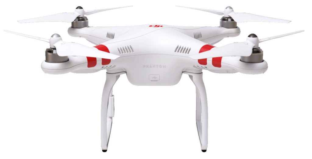
The main goal of this study is to show a step-by-step aero-acoustic benchmark validation of the DJI 9450 propeller. The simulation software used for this analysis is TCAE – a comprehensive simulation environment based on open source. The propeller that was investigated in this study, comes from real-world applications and is used to move drones. Particularly it is used on the popular civil drone DJI Phantom 3. This propeller was extensively measured in anechoic chambers and the measurement data are publicly available. The details about the noise measurements, methods, and facility descriptions, as well as other simulation results, can be found in the references [1,2,3]. This study shows a complete workflow of geometry preparation, simulation setup, simulation run, and results post-processing. The simulation results are compared with the measurement results.
Propeller DJI 9450 - Geometry Description
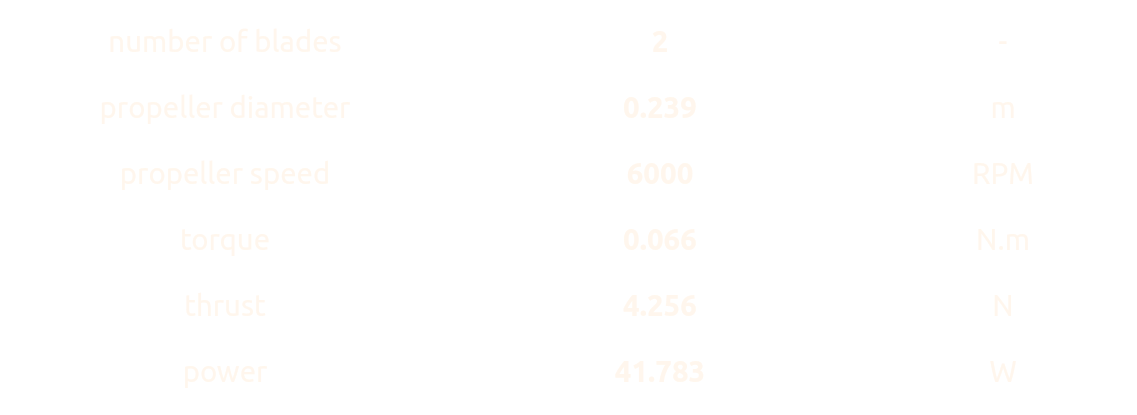
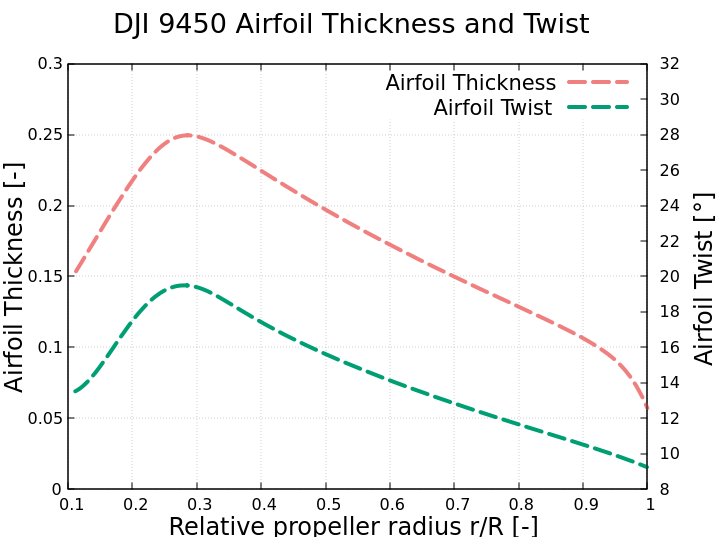
For several reasons the measurements were performed with a single propeller. The simulation has to mimic the measurements as much as possible, for the simulation, only a single propeller approach is used too. The propeller blade has its profile combined out of EPPLER 856 (0-0.2 r/R) and EPPLER 63 (0.2-1 r/R). The propeller had the following parameters:
Centrifugal Compressor - Simulation Input
A typical input for a detailed simulation analysis is a 3D surface model in form of an STL surface. For CFD simulation, it is needed to have a simulation-ready surface, which is a closed watertight model (sometimes also called waterproof, or model negative, or wet surface) of the model inner parts where the fluid flows. Similarly, for FEA simulation, it is needed to have a closed surface model of the solid of the impeller in form of a single STL surface.
Acoustic Analogy Theory
Acoustic analogies provide a way to calculate pressure fluctuations in a cheaper way than solving Navier-Stokes equations in very high resolution (the spatial resolution is so high that usage in real-world problems is almost impossible). There are several types of analogies from which the most common one is Ffowcs Williams-Hawkings with its Farassat1A formulation [4,5].
In short, the steps to get Ffowcs Williams-Hawkings equations are
Introduce a sound-producing surface. This can be a surface surrounding the noise source or the surface of the noise source directly (blades of a propeller, for example). In our case, it is a cylinder surrounding the rotation zone. Both the volume mesh and the surface mesh need to be fine enough, the rule of thumb is 25 cells on a wavelength to catch the corresponding frequency (frequency 1000 Hz requires a cell size of at least 0.01372 m).
Rearrange the fluid dynamics equations in such a way that we have a wave operator applied on pressure on the left-hand side and other quantities grouped in source terms on the right-hand side. The right-hand side now contains monopole (thickness) dipole (loading) surface sources and quadrupole volume sources. In our implementation, we neglect the quadrupole sources, which are the non-linear sources from turbulence. The monopole sources describe the noise generated by the displacement of fluid as the body passes. The dipole sources model the noise that results from the unsteady motion of the force distribution on the body surface.
Now we simplify the remaining terms. We use Green functions and rewrite time derivatives as space derivatives which give us the final equation p^prime(x,t) = p^prime_T(x,t) + p^prime_L(x,t),
where p^prime_T(x,t) is the thickness noise term
The symbols in equations (20.2) and (20.3) have the following meaning,
- f is the surface describing function.
- rho_zero is the reference density.
- r is the distance to the observer.
- Mr is the Mach number in the radiation direction.
- M is the magnitude of the local Mach number.
- c is the speed of sound.
- dot(v)_n = dot(v)_i * n_i , v_dot(n) = v_i * dot(n)_i , where v_i and n_i are the i-th components of velocity and surface normal vector, respectively.
- lr = li*ri where ri are components of the radiation direction vector and li are the components of local force intensity with Pij being the components of Lighthill compress tensor and uf is surface velocity.
- The subscript signalizes quantities evaluated in retarded time.
This list of steps is just to sketch where the equations came from and how they look. For a more detailed explanation see for example [6] and references therein.
Once the time series of acoustic pressure values are computed for each observer (the acoustic analogy simulation is finished), transformation to the frequency domain follows. As a result, we obtain the Sound Pressure Level and Power Spectral Density quantities for each observer. These quantities can be interpreted as a measure of the loudness of each tone (pressure fluctuation frequency) and overall loudness in the observer location.
This process we call Signal Processing consists of the following steps. At first, we clean the time signal from unwanted frequencies with the chosen signal filter (can be none, Butterworth, Chebyshev1, or Chebyshev2). These are standard types of signal filters and their implementation from the Python SciPy[7] library is used in TCAE. For more details search the internet, follow the references in [7] or ask your librarian.
The cleaned signal is then transformed to the frequency domain with Fourier Transform. In order to get reasonable results from acoustics the CFD results which play the role of input needs to be precise enough. If the CFD is of questionable quality, acoustic results cannot be good. Moreover, we want to use only the CFD data from times when the simulated flow is already stabilized (i.e., the first few rotations of a propeller simulation should be skipped). Then there is the time-step size t. We require CFD to be run with a fixed time step size. This is because the input to Fourier Transform is correct and the sampling frequency fs = 1 t is well-defined only for constant fixed t. The sampling frequency fs gives us a limitation for the accuracy of the signal processing results. The frequencies above Nyquist frequency fN = fs2 cannot be trusted (distorted by the aliasing effects).
If the signal is long enough more sophisticated treatment is possible. The so-called Welch method [8] splits the signal on a chosen number of (possibly overlapping) segments. On each segment, a window function is applied and the result is Fourier-transformed. Finally, the results of the segments are averaged which gives the final result.
The role of the window functions is to force the Fourier Transform to focus more on the data from the middle of the interval than on the corner values. The most important reason is the fact that the Fourier Transform silently assumes the last value matches the first value which is true for a perfectly periodic signal of the length of a whole number of periods but not true for real-life applications. This means not using any filter potentially leads to ill input to Fourier Transform. The window function properties and more information about them can be found for instance on the SciPy[7] website and references therein. Further reading on signal processing can be found in the example in [9].
With the Fourier Transform finished, we have the values for each considered frequency .
With this, we can calculate SoundPressure Level and Power Spectral Density quantities. They both describe “sound loudness” as a function of frequency . Their definitions and meanings are however not the same. The Sound Pressure Level for frequency is defined as
spl = 10*log(2*abs(fw))/(S*p0)
where is the reference sound pressure and is the normalization factor depending on the chosen window function.
The Power Spectral Density differs from the Sound pressure level in the aspects that it is a power so appears here in the second power and it is also a density, which we divide with sampling frequency . The equation is
PSD = 10*log(2fw)^2/(fsS2po^2)
where is (another) normalization factor depending on the chosen window function.
Propeller DJI 9450 - Simulation Input
A typical input for a detailed simulation analysis is a 3D surface model in the form of an STL surface, together with related physics and boundary conditions. For CFD simulation, it is needed to have a simulation-ready surface, which is a closed watertight model (sometimes also called waterproof, model negative, or wet surface) of the model’s parts where the fluid flows.
The input to the TCAA module out of TCAE software is fluid quantities evaluated on a reference surface (typically a cylinder or a sphere that surrounds the source of the noise). These quantities are density, pressure, and velocity and are collected during the CFD simulation run. In this particular case, the source surface (control surface) we used was a cylinder enclosing the propeller (including the rotating cylinder).
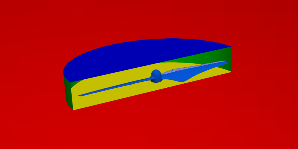
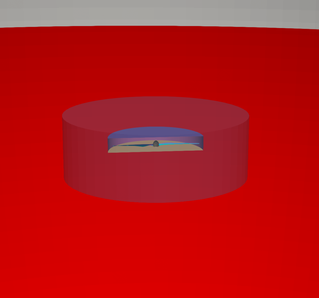
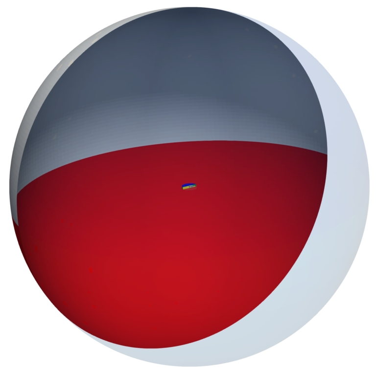
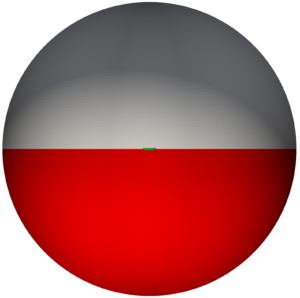
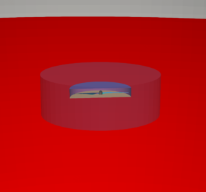
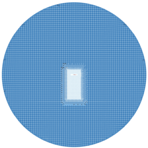
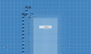
The propeller rotation method is solid body motion which means that the cylinder with a propeller inside is physically rotating in the simulation domain. The simulation domain is a sphere where technically the top hemisphere is an inlet and the bottom hemisphere is an outlet. The rotating cylinder (with a propeller inside) is rotating in the center of the sphere. The reference virtual surface (control surface) for acoustics data is a bigger cylinder (virtual – not part of the mesh!) and surrounds the smaller rotating cylinder.
Propeller DJI 9450 - CFD Preprocessing
For CFD simulation it is best to split the geometry into several waterproof components because of rotation (some parts may be rotating and others not). Each component itself has to be waterproof and consists of a few or multiple STL surfaces. It is smart to split each component into multiple surfaces (more is better) because it opens a broader range of meshing options, simulation methods (mesh refinements, manipulation, boundary conditions, evaluation of results on model-specific parts, …), and postprocessing.
The principle is always the same: the 3D surface model has to be created; all the tiny, irrelevant, and problematic model parts must be removed, and all the holes must be sealed up (a watertight surface model is required). This propeller CAD model is simple. The final surface model in the STL format is created as input for the meshing phase. This preprocessing phase of the workflow is extremely important because it determines the simulation potential and limits the CFD results.
In this drone propeller project, the CAD model was split into two logical parts: 1. The cylinder with the impeller blade inside. The cylinder is physically rotating. 2. The outer simulation domain – the sphere.
The surface model data in .stl file format together with physical inputs are loaded in TCFD. Another option would be loading an external mesh in OpenFOAM mesh format or loading an MSH mesh format (Fluent mesh format), or CGNS mesh format. This CFD methodology employs a multi-component approach, which means the model is split into a certain number of components. In TCFD each region can have its own mesh and individual meshes communicate via interfaces.
Propeller DJI 9450 - CAA Preprocessing
As mentioned above, the input to the TCAA module needs certain CFD fields evaluated on a reference surface (control surface). We chose to use a cylinder that encloses the propeller together with the rotational domain (smaller cylinder). The values need to be stored for several time steps and fixed time-step-size in the CFD simulation is required as we need the input to Fourier transform to have equal stepping in time. The location of the source surface (control surface) matters, we need to catch the values of CFD fields close enough to the propeller where the mesh is finer because the results are more accurate here.
On the other hand, we need all the sources to be inside the source surface (control surface), this talks about keeping the cylinder further away from the propeller. Mankbadi et al., in [1] came to the conclusion that the suitable radius for the control cylinder is 1.2 times the propeller radius. Another aspect that can influence the results’ accuracy is the surface resolution. The finer the resolution is the more accurate the results are. At least in theory. But having the surface resolution higher than the local CFD mesh coarseness will, of course, not help us. In TCAE software, the acoustic control surface can either be created with chosen shape, location and resolution, or an external STL file can be used. As a third option, CFD patches can be used too.
IMPORTANT NOTICE ON PREPROCESSING
The surface of the simulation-ready model has to be clean, simple enough but not simpler! The principles are always the same: the watertight surface model has to be created; all the tiny, irrelevant, and problematic model parts must be removed, and all the holes must be sealed up (the watertight surface model is required). The preprocessing phase is an extremely important part of each simulation workflow. It sets up all the simulation potential and limitations. It should never be underestimated. Mistakes or poor quality engineering in the preprocessing phase can be hardly compensated later in the simulation phase and postprocessing phase. For more details, see the TCAE documentation.
Propeller DJI 9450 - CFD Meshing
The computational mesh for CFD is created in an automated software module TMESH, using the snappyHexMesh open-source application. All the mesh settings are done in the TCAE GUI.
For each model component, a cartesian block mesh is created (box around the model), as an initial background mesh, that is further refined along with the simulated object. The basic mesh cell size is a cube defined with the keyword “background mesh size“.
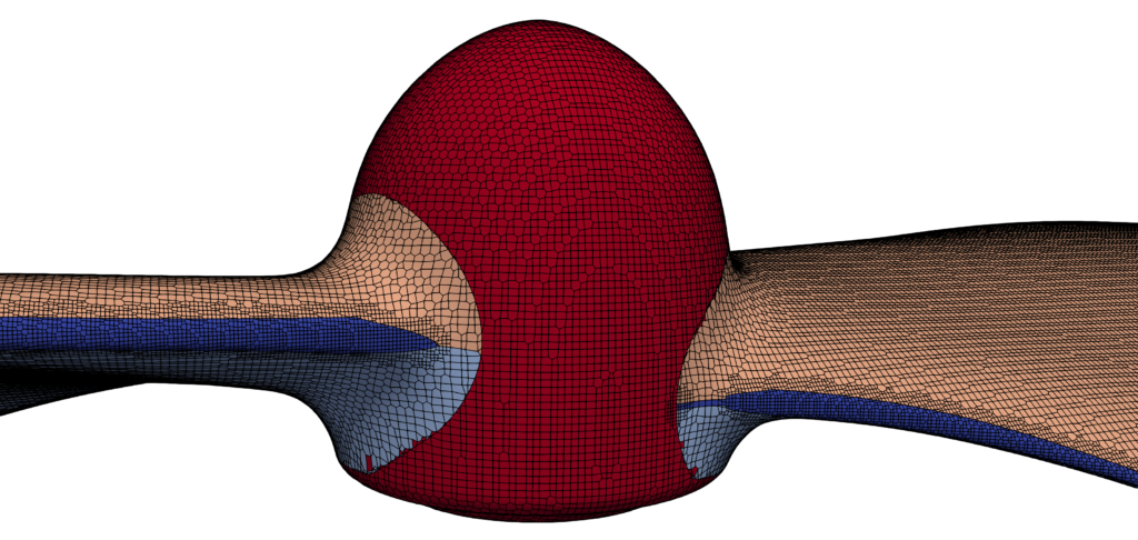
The mesh is gradually refined to the model wall. The mesh refinement levels can be easily changed, to obtain the coarser or finer mesh, to better handle the mesh size. Inflation layers can be easily handled if needed. As already stated, one of the key things to perform a good CAA simulation is a choice of a representative control surface. Its properties were described in the previous section. The generation of the control surface is executed in GMSH meshing software with desired shape and accuracy specified.
The total number of mesh cells is always a big question for every CFD project. In this particular case, we run several meshes with the various number of mesh cells, varying from 2 million to 12 million with no major effect on the results. However, the proper mesh (grid) dependence study should be done. In this project, the authors only follow the basic analysis that the smallest cell should be smaller than 0.013 m. The exact mesh settings remain the object of future investigation.
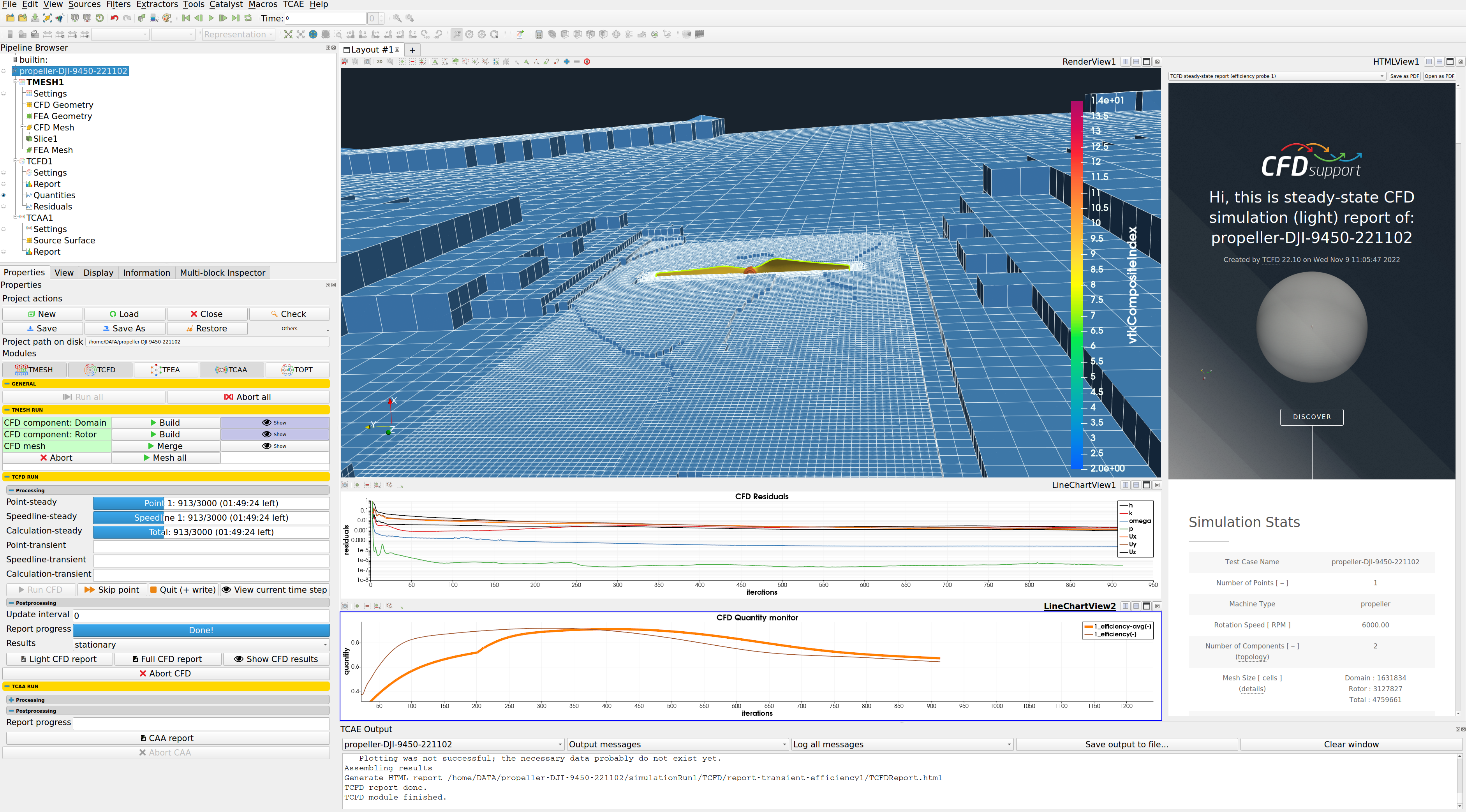
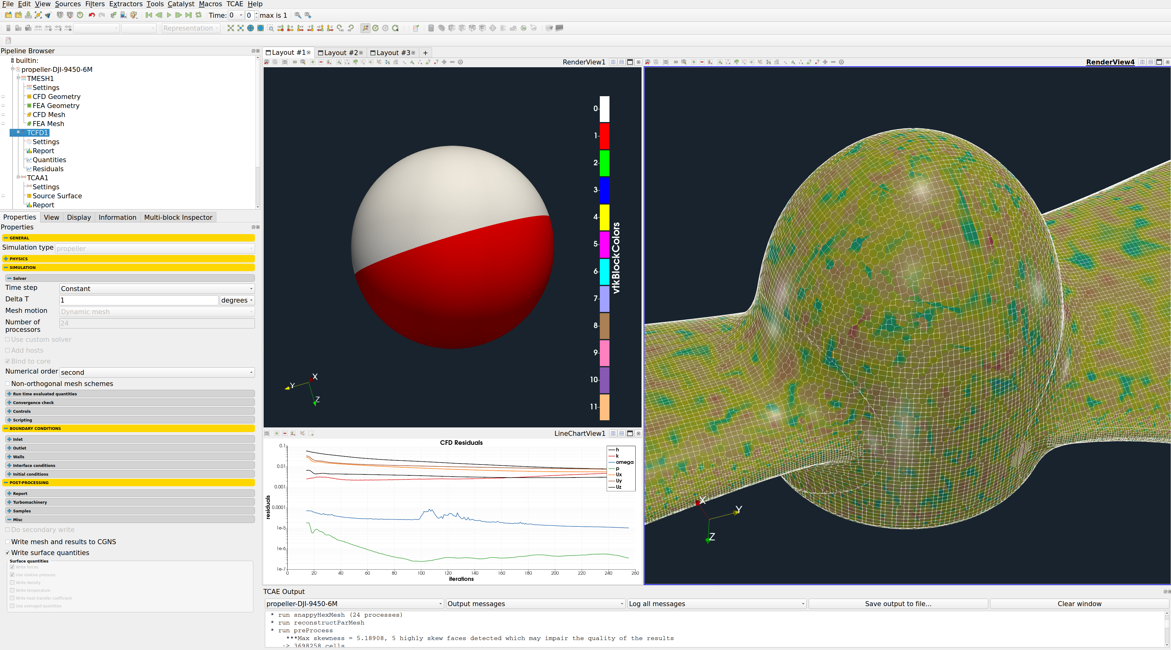
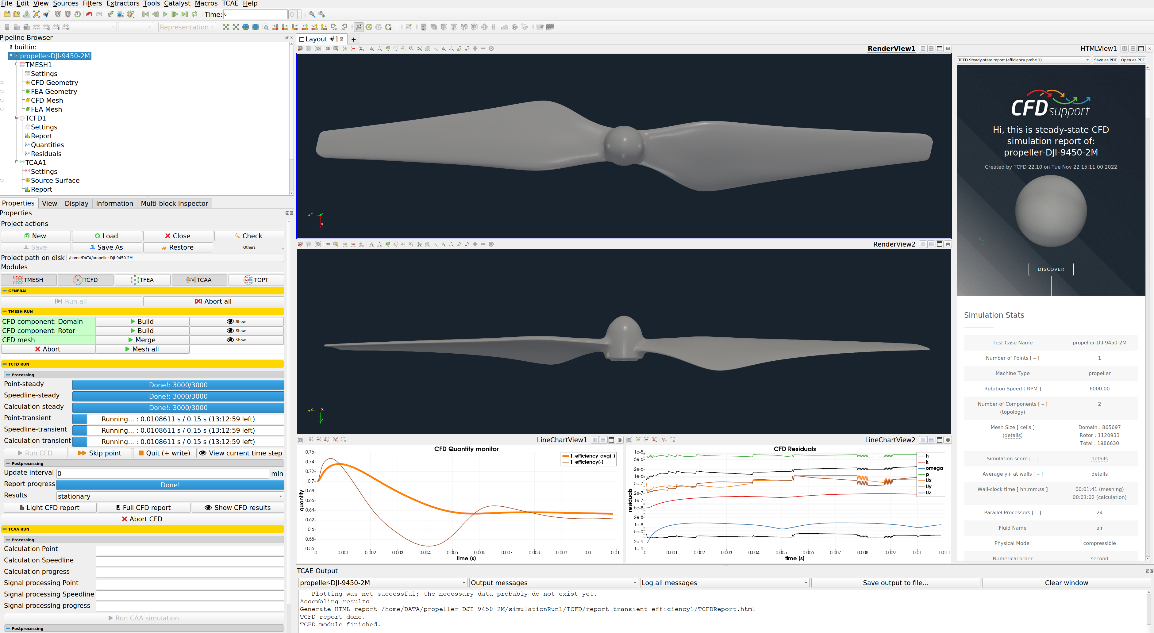
CFD Simulation Setup
The CFD simulation is managed with the TCAE software module TCFD. Complete CFD simulation setup and run are done in the TCFD GUI in ParaView. TCFD is based on the OpenFOAM open-source software. The simulation setup is done in GUI from the top menu to the bottom.
- Simulation type: propeller
- Time management: transient
- Physical model: Compressible
- Number of components: 2 [-]
- Wall roughness: none
- Speed: 6000 [RPM]
- Outlet: variable static pressure [m2/s2]
- Turbulence: URANS
- Turbulence model: k-omega SST
- Shear Thinnig model: Newtonian
- Wall treatment: Wall functions
- Turbulence intensity: 5%
- Speedlines: 1 [-]
- Simulation points: 1 [-]
- Fluid: Air
- Reference pressure: 1 [atm]
- Dynamic viscosity: 2.144 × 10E-5 [Pa⋅s]
- Reference density: 1.2 [kg/m3]
- CFD CPU Time: min 25 core.hours/point/round
- BladeToBlade: on
Propeller DJI 9450 - CAA Simulation Setup
The CAA simulation is managed with the TCAE software module TCAA. Complete CAA simulation setup and run are done in the TCAA GUI in ParaView. TCAA is based on the libAcoustics OpenFOAM library [10]. This library was hugely adjusted to fit the TCAE family in the best possible way. The biggest difference is TCAA uses data from disk so one set of data can be used repeatedly for more CAA simulations. In contrast, the original libAcoustics library works in the OpenFOAM run time with temporal data.
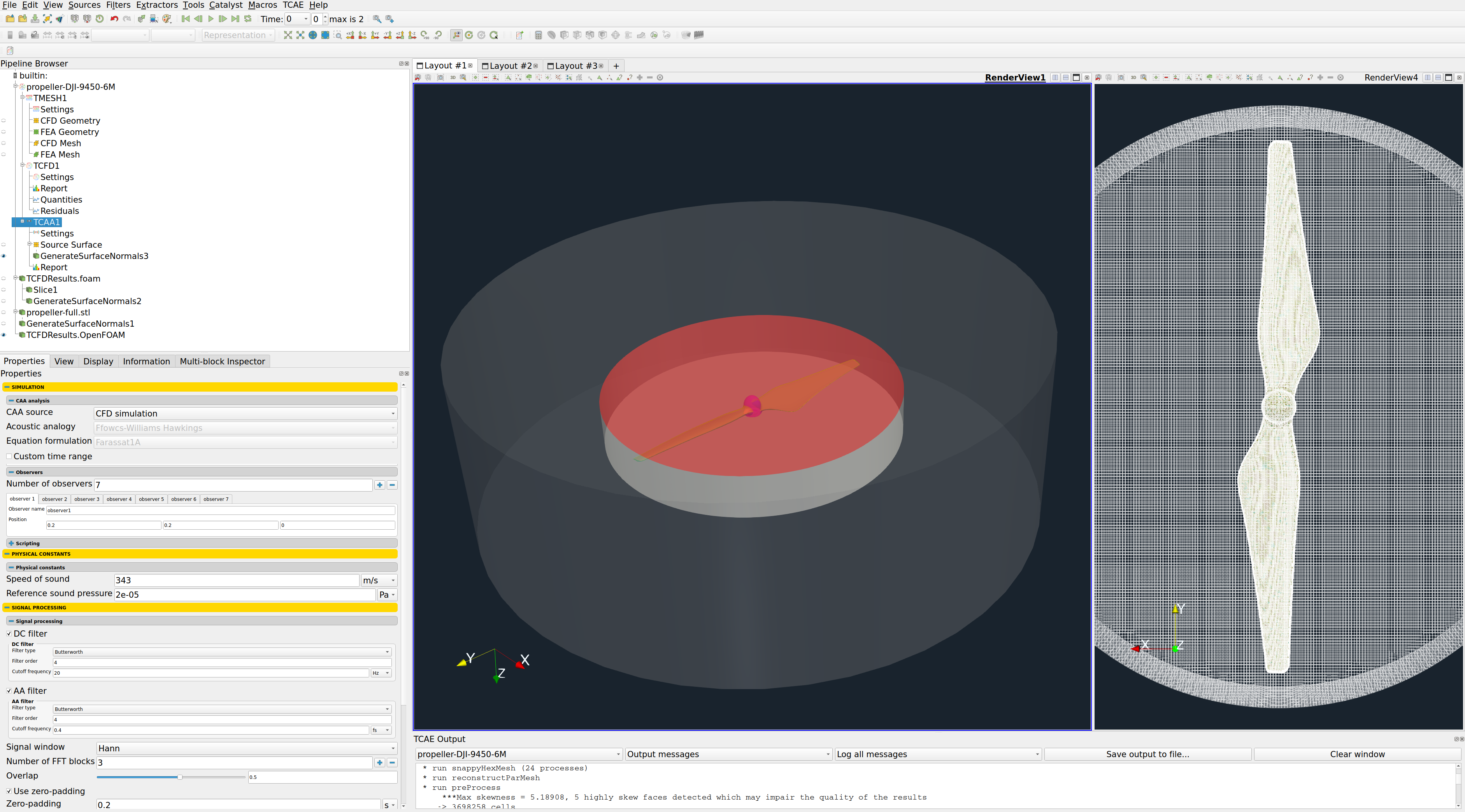
Once the time evolution of acoustic pressure for all observers is computed the signal processing comes to play. TCAA uses Python script with SciPy functions to convert the temporal signal to the frequency domain. The first step of the signal processing step is filtering the signal to clean it from high frequencies that can cause unwanted aliasing phenomena, as well as from low frequencies (DC shift). A clean temporal signal serves as input to the Fourier transform and subsequently, Power Spectral Density and Sound Pressure Level are computed.
- Speed of sound: 343 [m/s]
- Signal source: TCFD [-]
- Reference pressure: 1 [atm]
- Material density: 7800 kg/m3
- Medium:: Air [-]
- Acoustic Analogy: Ffowcs Williams-Hawkings [-]
- Formulation: Farassat 1A [-]
- Reference sound pressure: 2e-5 [Pa]
- Speed of rotation: 6000 [RPM]
Propeller DJI 9450 - TCAE Simulation
The TCAE simulation run is completely automated. The whole workflow can be run by a single click in the GUI, or the whole process can be run in batch mode on a background. Modules used in this particular project are TMESH, TCFD, and TCAA The simulation is executed in the transient mode.
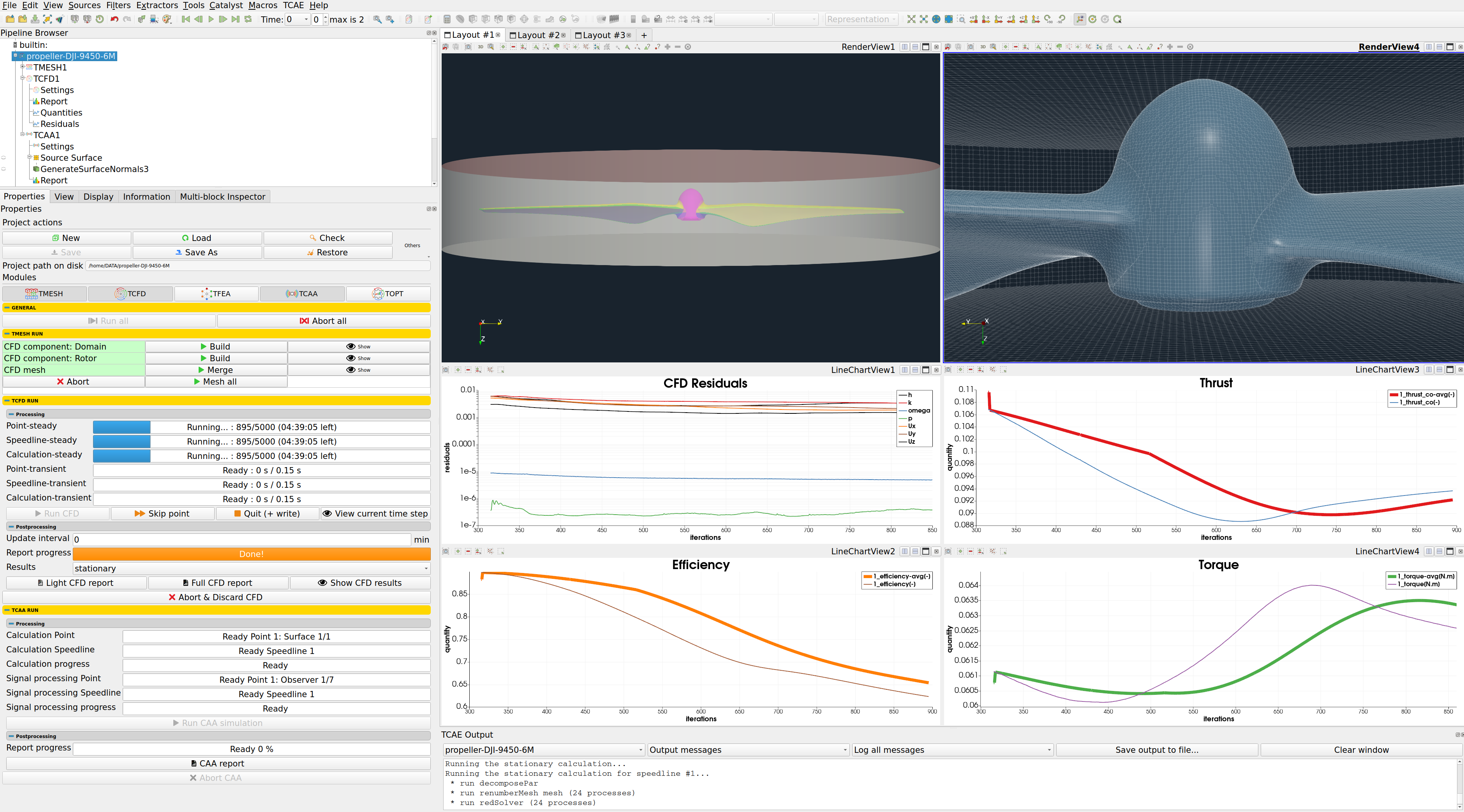
TCFD includes a built-in post-processing module that automatically evaluates all the required quantities, such as efficiency, torque, forces, force coefficients, flow rates, pressure, velocity, and much more. All these quantities are evaluated throughout the simulation run, and all the important data is summarized in an HTML report, which can be updated anytime during the simulation, for every run.
All the simulation data are also saved in tabulated .csv files for further evaluation. TCFD is capable of writing the results down at any time during the simulation. The convergence of basic quantities and integral quantities are monitored still during the simulation run. The geometry was created one-time using TCAD in the preprocessing phase. First, the TMESH is executed to create the volume mesh for CFD. Then the CFD simulation is executed and evaluated with fields needed for acoustic being stored on the source surface. Once the CFD simulation is finished, the CAA simulation starts, first the acoustic pressure for each observer is calculated and then the Sound Pressure Level and Power Spectral Density are computed, again for each observer separately.
Propeller DJI 9450 - Post-processing - Integral Results
The integral results and simulation statistics are evaluated automatically for every simulation run. Every simulation run in TCAE has its own unique simulation report. The integral results both for CFD and FEA are written down in the corresponding HTML or PDF reports.
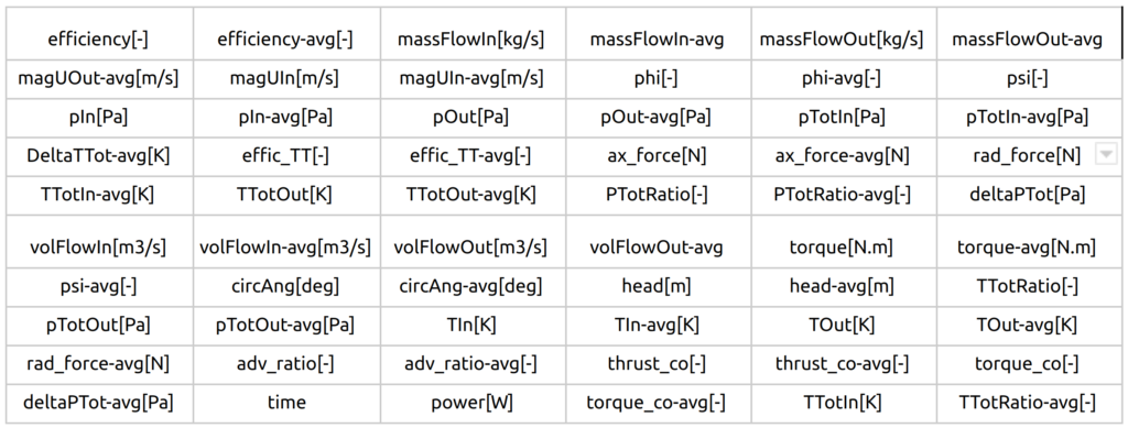
All the relevant integral quantities are evaluated, sorted, and stored in the corresponding CSV files and are ready for further usage. The following integral quantities are evaluated every time step.
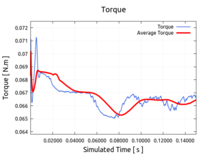
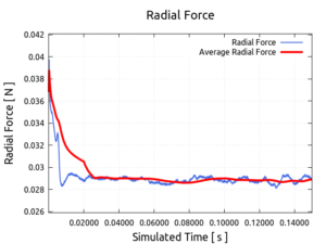
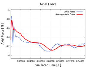
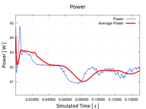
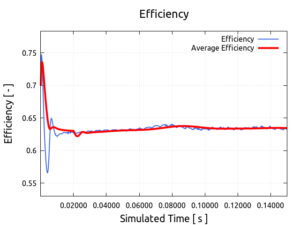
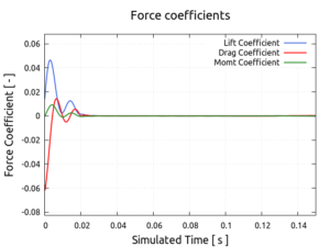
All the relevant integral quantities are evaluated, sorted, and stored in the corresponding CSV files and are ready for further usage. Following integral quantities are evaluated every time step.
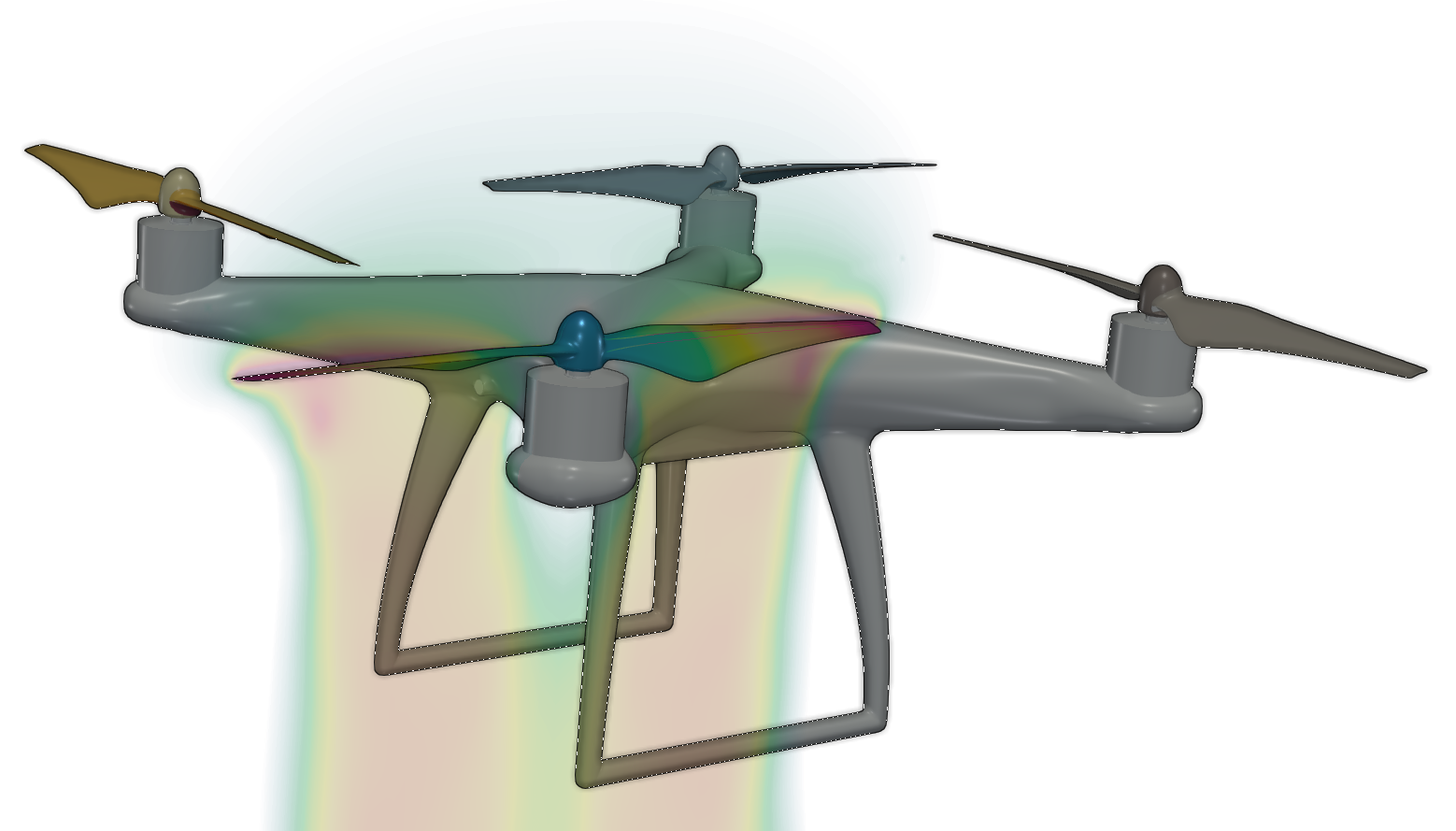
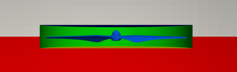
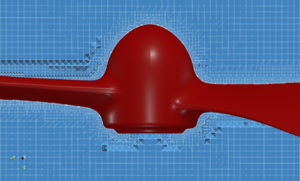
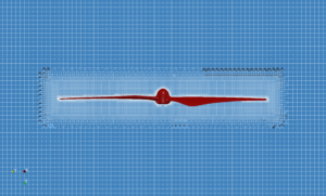
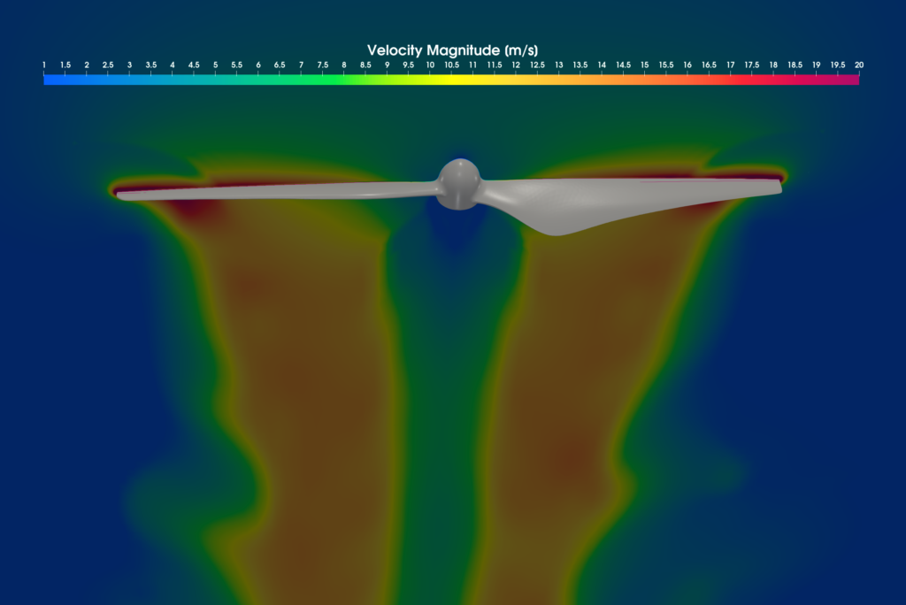
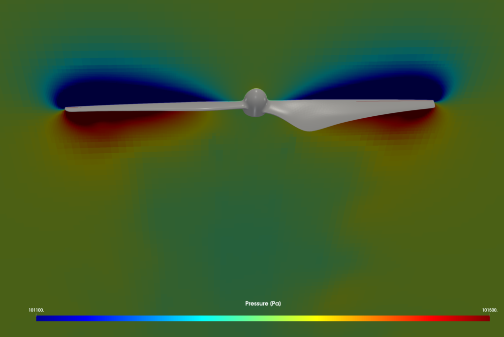
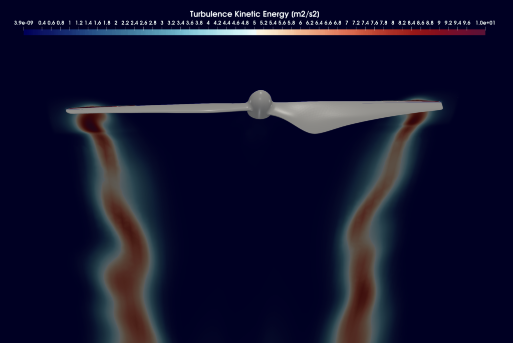
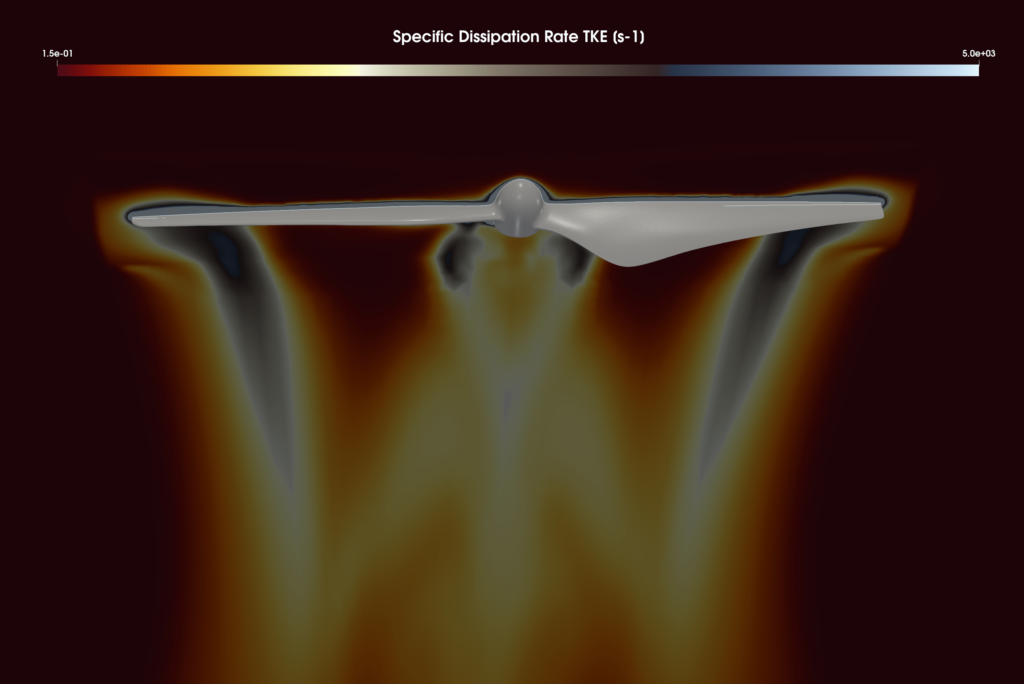
Propeller DJI 9450 - Postprocessing - CFD Volume Fields
While all the integral results are stored in the CSV files and are available for further postprocessing, the volume fields are post-processed in the open-source visualization tool ParaView. ParaView provides a wide range of tools and methods for CFD & FEA postprocessing and results evaluation. There are available countless useful filters and sources, for example, Calculator, Contour, Clip, Slice, Threshold, Glyph (Vectors), Streamtraces (Streamlines), and many others.
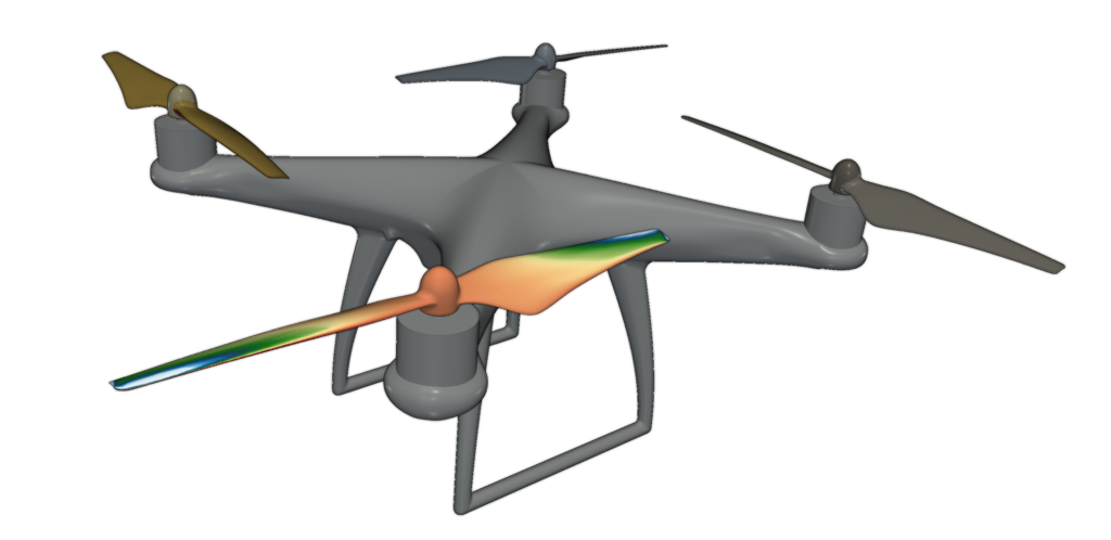
CFD Volume Fields
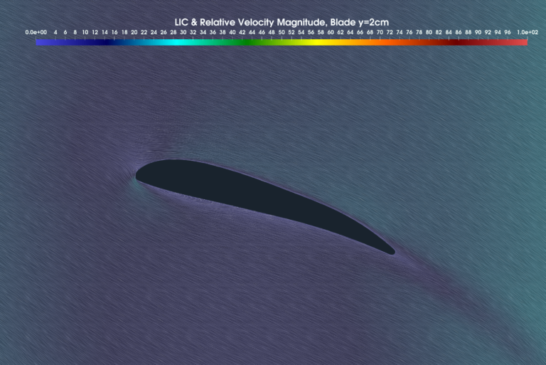
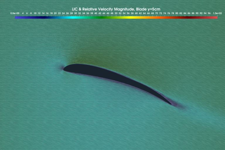
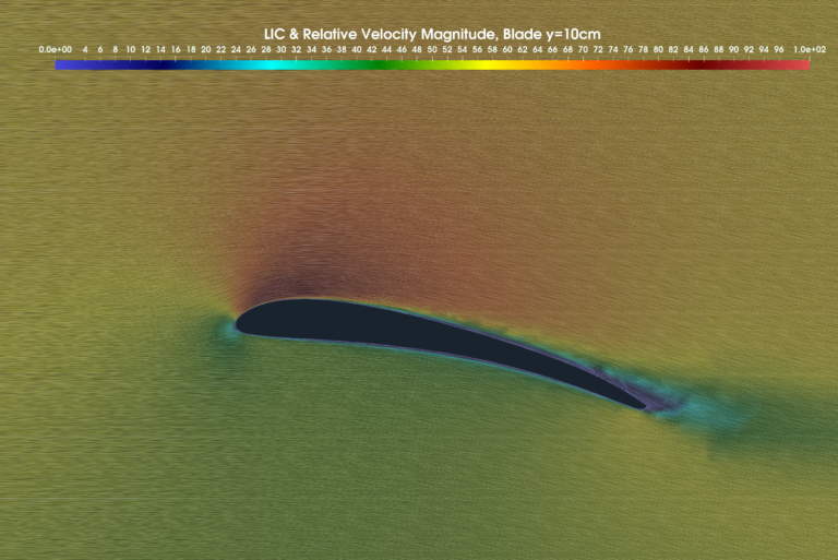
CFD Blade to Blade View
Propeller DJI 9450 - Acoustic Results
The most useful CAA results are the acoustic quantities in the observer position. These are the temporal evolution of acoustic pressure and Sound Pressure Level and Power Spectral Density. All this is part of the CAA HTML report in the form of plots and tables.
In this paper, we present graphs for the observer located in a position [0.128, 1.423, 0.779] with the origin being the center of the propeller and the axis of rotation the z axis pointing downwards. This should correspond to the measurement and observer of the location from the papers [1,2].
Propeller DJI 9450 - Acoustic Results
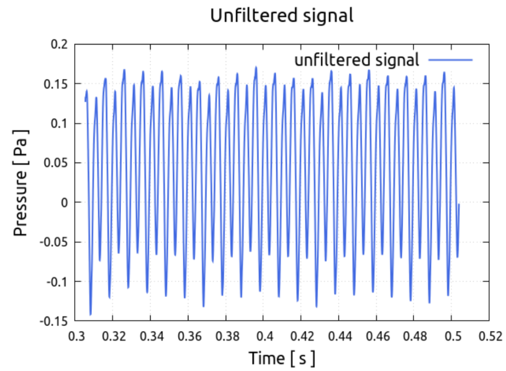
The graph titled “Unfiltered signal” is the result of the Acoustic Analogy simulation. It is the raw sound pressure evolution in the observer position. We can see here that we used data from 0.3 s to 0.5 s of the simulation time. In the language of propeller revolutions, this corresponds to 30-50 revolutions. The data from the first 30 revolutions are not used for acoustic investigations. In the TCAA workflow, the signal is later cleaned with signal filters.
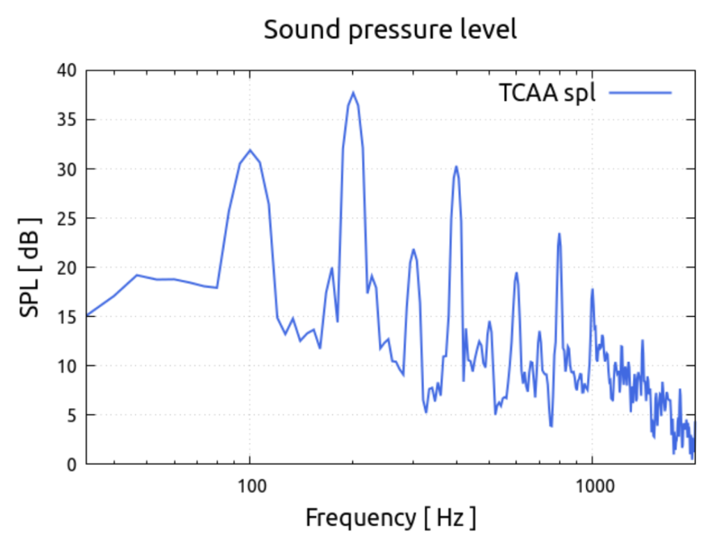
The graphs “Power spectral density” and “Sound pressure level” depict the frequency domain quantities calculated from the Fourier-Transformed temporal signal. Their definitions are stated in the chapter Signal Processing Theory, for the equations we kindly refer to there or to the literature.
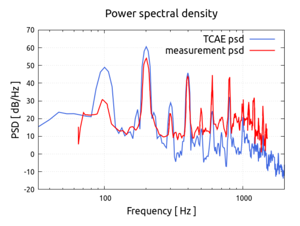
For the power spectral density, we also show the results from the references [1,2] (red line) compared to ours (blue line). We see that our model correctly recognizes the blade passage frequency (bpf = rotations per second # blades = 100 2 = 200 Hz) as the loudest frequency. The multiples of bpf are also caught as peaks. Although we meet quite a good agreement with the reference we still observe differences in the magnitudes. This can be caused by several reasons: we might use different propeller geometry than Mankbadi et al.,[2] use in their study. Despite visually being similar and also similar to the real measured propeller, subtle diversities can cause different results. The exact location of the observer is questionable too as in the original paper it is described with the respect to the center of the drone, not to the center of the propeller as we need it, and the dimensions of the drone needed to be estimated.
We also need to mention that the simulation of Mankbadi et al.,[2] which we compare to and is almost indistinguishable from the measurements, is way more expensive than ours. The mesh size is 70 million cells compared to ours 5 million, time step size of about 0.025° rotor rotation (approx. 7.510-9 s) compared to our 1° rotor rotation (approx. 2.710-5 s). We both started to use data at the simulation time 0.3 s whereas we use only 0.2 s long time interval, Mankbadi et al.,[2] use 0.5 s long interval. Taking these notes into account we can conclude the light-weighted TCAE simulation predicts correctly the acoustic behavior of DJI propeller 9450.
Conclusion
- It has been shown how to make a comprehensive CFD & CAA analysis of the real-world propeller in a single automated workflow.
- The TCAE results were successfully compared to the measurement data.
- There was no special tweaking used in the CFD simulation at all.
- There remains a lot of space for tuning the CFD methodology, especially for the mesh resolution, turbulence modeling, and numerical schemes.
- TCAE showed to be a very effective tool for CFD, FEA, and FSI engineering simulations for all rotating machinery in general.
- This benchmark study was intentionally written in short not to overwhelm its readers with too many details.
- The original intention was to show the modern simulation workflow and its potential.
- The benchmark details are listed in the references below.
- All the technical details regarding CFD & CAA simulation are listed in the TCAE manual.
- The benchmark geometry and data are freely available for download on the CFDSUPPORT website https://www.cfdsupport.com.
- More information about TCAE can be found on the CFD SUPPORT website: https://www.cfdsupport.com/tcae.html
- Questions will be happily answered via email info@cfdsupport.com
Acknowledgement
Special thanks of gratitude to all technical advisors, especially to Mats Gustavsson and Prof. Sofiane Khelladi who helped CFDSUPPORT to understand a lot of issues associated with acoustics and signal processing.
References
[1] Intaratep, N., Alexander, W.N., Devenport, W.J., Grace, S.M., Dropkin, A. (2016) Experimental Study of Quadcopter Acoustics and Performance at Static Thrust Conditions, 22nd AIAA/CEAS Aeroacoustics Conference.
[2] Mankbadi, R.R., Afari, S.O., and Golubev, V.V (2020) Simulations of Broadband Noise of a Small UAS’ Propeller, 10.2514/6.2020-1493.
[3] Zawodny, N.S., Boyd, D.D., and Burley, C.L. (2013) Acoustic Characterization and Prediction of Representative, Small-Scale Rotary-Wing Unmanned Aircraft System Components, Proceedings of the American Helicopter Society 72nd Annual Forum.
[4] Glegg, S. and Devenport, W. (2017) Aeroacoustics of Low Mach Number Flows, Academic Press
[5] Farassat, F. (2007) Derivation of Formulations 1 and 1A of Farassat
[6] Brentner, K.S., Farassat, F. (2003) Modeling aerodynamically generated sound of helicopter rotors, Progress in Aerospace Sciences, Volume 39, Issues 2–3
[7] Virtanen, P., Gommers, R., Oliphant, T.E., Haberland, M., Reddy, T., Cournapeau, D., Burovski, E., Peterson, P., Weckesser, W., Bright, J., van der Walt, S. J., Brett, M., Wilson, J., Millman, K.J., Mayorov, Nelson, A.R.J., Jones, E., Kern, R., Larson, E., Carey, C.J., Polat, İ., Feng, Y., Moore, E.W., VanderPlas, J., Laxalde, D., Perktold, J., Cimrman, R., Henriksen, I., Quintero, E.A., Harris, Ch.R., Archibald, A.B., Ribeiro, A.H., Pedregosa, F., van Mulbregt, P., (2020) SciPy 1.0: Fundamental Algorithms for Scientific Computing in Python. Nature Methods, 17(3), 261-272.
[8] Welch, P.D. (1967) The Use of Fast Fourier Transform for the Estimation of Power Spectra: A Method Based on Time Averaging Over Short, Modified Periodograms, IEEE Transactions on Audio and Electroacoustics, vol. 15, no. 2, pp. 70-73, doi: 10.1109/TAU.1967.1161901.
[9] Heinzel, G., Rüdiger, A. and Schilling R. (2002) Spectrum and spectral density estimation by the Discrete Fourier transform (DFT), including a comprehensive list of window functions and some new flat-top windows.
[10] Epikhin, A., Evdokimov, I., Kraposhin, M., Kalugin, M., Strijhak, S. (2015) Development of a Dynamic Library for Computational Aeroacoustics Applications Using the OpenFOAM Open Source Package, Procedia Computer Science, DOI: 10.1016/j.procs.2015.11.018
[11] Moslem, F., Masdari, M., Fedir, K., Moslem, B., 2022/08/02, SP – 095441002210913, Experimental investigation into the aerodynamic and aeroacoustic performance of bioinspired small-scale propeller planforms, DO – 10.1177/09544100221091322, JO – Proceedings of the Institution of Mechanical Engineers, Part G: Journal of Aerospace Engineering
[12] TCAE Training – https://www.cfdsupport.com/download-documentation.html
[13] TCAE Manual – https://www.cfdsupport.com/download-documentation.html
[14] TCAE Webinars – https://www.youtube.com/playlist?list=PLbxC_ERCZDHbytN1WvSRi57eksKTNtTis
Download TCAE Tutorial - Propeller DJI 9450 Benchmark
File name: propeller-DJI-9450-TCAE-Tutorial.zip
File size: 28 MB
Tutorial Features: CFD, CAA, TCAE, TMESH, TCFD, SIMULATION, PROPELLER, TURBOMACHINERY, COMPRESSIBLE FLOW, COMPRESSIBLE, URANS, STEADY-STATE, AUTOMATION, WORKFLOW, RADIAL FLOW, SEGMENT, SNAPPYHEXMESH, NETGEN, 5 COMPONENTS, RPM=6000, D=239mm