Labyrinth Seal - Multiphase VoF
This case study presents a multiphase CFD simulation of a labyrinth seal using the Volume of Fluid (VoF) method. The setup demonstrates the capability of the simulation framework to handle transient multiphase flows in complex internal geometries.
This case serves as a showcase example of multiphase VoF simulations applied to engineering geometries, demonstrating the capability to simulate pressure-driven multiphase flow in complex internal geometries.
Geometry Description & CFD Preprocessing
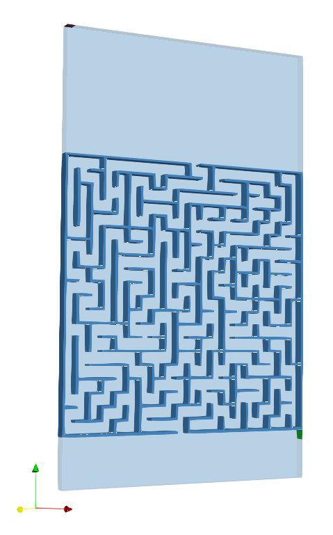
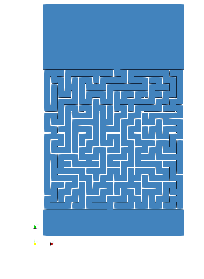
The computational domain represents a labyrinth seal geometry. The geometry consists of the labyrinth region itself together with the surrounding wall.
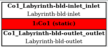
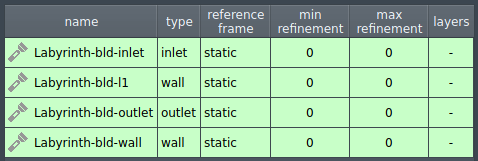
Within the wall boundaries, two main boundary patches are defined: an inlet and an outlet. The inlet, highlighted in red in the accompanying figure, represents the location where the total pressure boundary condition is applied. The outlet, marked in green, is defined as the downstream boundary where a fixed static pressure is prescribed. These boundary patches are used later in the simulation setup to define the pressure-driven flow through the labyrinth structure.

CFD Meshing
The computational mesh is generated from a background mesh with a base cell size of 0.007 m, which defines the overall resolution of the domain. Both the minimum and maximum surface refinement levels are set to zero in order to keep the mesh relatively coarse and computationally inexpensive for the purposes of this tutorial.
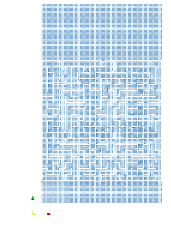
To ensure that the sharp geometric features of the labyrinth seal are still captured despite the limited refinement, feature edge detection and snapping techniques are employed. Feature edges are extracted from the STL geometry using an included angle criterion, which allows the identification of sharp corners and edges in the geometry. Additionally, the surfaceHookUp option can be enabled to improve the connectivity of feature edges.
During mesh snapping, both implicit and explicit feature snapping methods are activated. These methods help align the mesh with the detected feature edges and improve the resolution of sharp corners. Additionally, multiple feature snapping iterations are performed to progressively adjust the mesh towards the geometric edges.
CFD Simulation Setup
The CFD simulation is performed using the TCFD module, part of the TCAE simulation framework. The entire CFD simulation setup and execution are carried out through the TCFD GUI integrated within ParaView. TCFD uses OpenFOAM open-source application.
The simulation is performed as a transient, incompressible flow using a two-phase Volume of Fluid (VoF) approach to model water and air. The water phase is defined as the primary phase, while air is treated as the secondary phase with its own fluid properties.
The primary phase (air) is specified under Physics: Fluid Properties. The secondary phase (water) is activated by enabling Multiphysics: Multiphase VoF, where its fluid properties (name, density, viscosity) are defined. In addition, surface tension between the two phases is specified within the VoF settings.
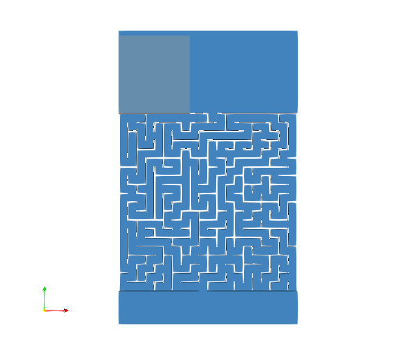
Initial phase distribution is prescribed in Boundary Conditions: Initial Conditions, where the second-phase volume is defined. By default, the entire domain is initialized with the first phase, and the second phase is then assigned to selected regions based on the specified second-phase volumes. In this case, the second phase is initialized using a two box-shaped volumes, although other shapes such as sphere or cylinder can also be used.
Volume 1 – Box (water)
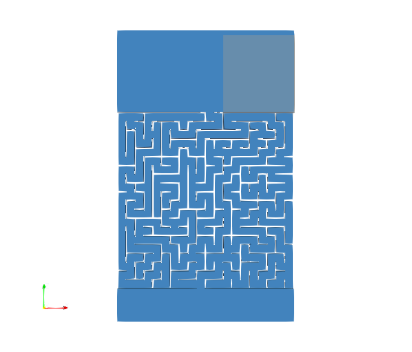
Volume 2- Box (water)
- TCAE Simulation type: general
- Number of components: 1 [-]
- Speedlines: 1 [-]
- Simulation points: 1 [-]
- Wall roughness: none
- Turbulence: k-ω-SST
- Wall treatment: Wall functions
- Time management: Transient
- Time step: constant, 0.0002s
- Dynamic Mesh
- Physical run-time: 30 s
- Physical model: Incompressible
- Gravity
- Multiphase VoF
- Surface tension: σ=0.07
- Primary phase: Air
- density: ρ = 1.2 kg/m3
- viscosity: μ = 1.8 e-5 Pa s
- Secondary phase: Water
- density: ρ = 1000 kg/m3
- viscosity: μ = 0.001 Pa s
The flow is driven by prescribed pressure boundary conditions. At the inlet total pressure is set to 1 atm, while the outlet is defined by a fixed static pressure of 1 atm.
Turbulence is modeled using the k–ω SST model, with standard wall functions applied at all walls, and all solid boundaries are treated as no-slip walls. The influence of gravity is also included in the simulations.
An constant time step Δt = 0.0002s is employed.
The case is configured to run for a physical time of 60 s.
The computational setup includes one speedline and one simulation point.
Pressure–velocity coupling is handled using the PIMPLE algorithm.
Tips
The setup follows recommended practices commonly used in VOF tutorial cases, where certain options are intentionally disabled to improve solver robustness in transient multiphase simulations.
- In particular, the velocity gradient caching option is disabled. This setting is recommended because enabling it may lead to instability or solver crashes during parallel computations. For this reason, it is considered best practice in similar tutorial cases to keep this option turned off.
- Additionally, the momentum predictor inside the PIMPLE loop is also disabled. This configuration follows the recommendations used in standard VOF tutorial setups, where disabling the momentum predictor can improve stability in transient simulations involving complex flow behavior.
Postprocessing
Download TCAE Tutorial - labyrinth
File name: labyrinth-TCAE-Tutorial.zip
File size: 8 MB
Tutorial Features: CFD, TCAE, TMESH, TCFD, SIMULATION, INCOMPRESSIBLE FLOW,TRANSIENT, k-ω-SST,AUTOMATION,WORKFLOW, MULTIPHASE, Volume of Fluid, VOF, 3D, Finite Volume, CFD, SnappyHexMesh,TCAE environment, OpenFOAM, k-ω-SST