1

Previous: addLayersControls Up: SnappyHexMesh mesh Next: snappyHexMesh log

This is an automatically generated documentation by LaTeX2HTML utility. In case of any issue, please, contact us at info@cfdsupport.com.

meshQualityControls

This block holds mesh quality parameters and their thresholds. During the mesh generation, the quality measurement is performed and quality parameters are evaluated. If mesh quality parameters exceeds the defined thresholds the algorithm try to re-apply the offending changes in the next iteration loop.


  • A brief explanation of mesh quality parameters can be found in the snappyHexMeshDict.
    //- Maximum non-orthogonality allowed. Set to 180 to disable.
    maxNonOrtho 65;
    
    //- Max skewness allowed. Set to <0 to disable.
    maxBoundarySkewness 20;
    maxInternalSkewness 4;
    
    //- Max concaveness allowed. Is angle (in degrees) below which concavity
    //  is allowed. 0 is straight face, <0 would be convex face.
    //  Set to 180 to disable.
    maxConcave 80;
    
    //- Minimum pyramid volume. Is absolute volume of cell pyramid.
    //  Set to a sensible fraction of the smallest cell volume expected.
    //  Set to very negative number (e.g. -1E30) to disable.
    minVol 1e-16;
    
    //- Minimum quality of the tet formed by the face-centre
    //  and variable base point minimum decomposition triangles and
    //  the cell centre. Set to very negative number (e.g. -1E30) to
    //  disable.
    //     <0 = inside out tet,
    //      0 = flat tet
    //      1 = regular tet
    minTetQuality -1e+20;
    
    //- Minimum face area. Set to <0 to disable.
    minArea 1e-13;
    
    //- Minimum face twist. Set to <-1 to disable. dot product of face normal
    // and face centre triangles normal
    minTwist 0.02;
    
    //- Minimum normalised cell determinant. This is the determinant of all
    //  the areas of internal faces. It is a measure of how much of the
    //  outside area of the cell is to other cells. The idea is that if all
    //  outside faces of the cell are 'floating' (zeroGradient) the
    //  'fixedness' of the cell is determined by the area of the internal faces.
    //  1 = hex, <= 0 = folded or flattened illegal cell
    minDeterminant 0.001;
    
    //- Relative position of face in relation to cell centres (0.5 for orthogonal
    //  mesh) (0 -> 0.5)
    minFaceWeight 0.02;
    
    //- Volume ratio of neighbouring cells (0 -> 1)
    minVolRatio 0.01;
    
    //- Per triangle normal compared to average normal. Like face twist
    //  but now per (face-centre decomposition) triangle. Must be >0 for Fluent
    //  compatibility
    minTriangleTwist -1;


  • The most important quality metrics:
    • orthogonality – is the angular deviation of the vector connecting two cell centers and the surface normal vector of their common face (see Figure below)
ortogonality

Figure: Orthogonality.

skewness – is defined as 38, where 39 is the distance between the common face center (black dot) and intersection of the common face and line connecting the cell centers (red dot); $ \vert\vec p\vert$ is the distance between te cell centers (see Figure below).
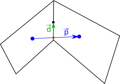
skewness

Figure: Skewness.

 
  • aspect ratio – is defined as the ratio of the maximum side of the cell ($ \Delta x$) and the minimum side ($ \Delta y$), see Figure below.
aspectRatio

Figure: Aspect ratio.

Solvers

  • Solvers are executable applications for numerical simulations of Computational Fluid Dynamics
  • Source code of solvers is located in the path of system variable $FOAM_SOLVERS
  • You can jump to the OpenFOAM solvers directory e.g using system variable
    $FOAM_SOLVERS:
    # cd $FOAM_SOLVERS
  • You can jump to the OpenFOAM solvers directory e.g using alias sol:
    # sol
    # ll
  • Basic types of solvers:

    basicpotential flow, Laplace and transport equations
    combustioncombustion fluid flows
    compressiblecompressible fluid flows
    discreteMethodsmolecule movement
    DNSdirect numerical simulations
    electromagneticselectrostatics, magnetohydrodynamics
    financialBlack-Scholes equation to price commodities
    heatTransferheat transfers flows
    incompressibleincompressible flows
    lagrangianLagrangian approach to CFD
    multiphasemultiphase flows
    stressAnalysisstress analysis in a solid body

Previous: Example: Blade pressure and Up: Example: Blade pressure and Next: Meridional Average filter –
This is an automatically generated documentation by LaTeX2HTML utility. In case of any issue, please, contact us at info@cfdsupport.com.

Step by step guide

Step 1 — Load the rotor part of an OpenFOAM case into ParaView using the command paraFoam -region rotor. Avoid loading the whole mesh; choose only the blade walls and the hub and shroud patches. Choose some non-zero simulation time, select appropriate components (“Mesh parts”) and fields (“Volume fields”) and press “Apply”. This will load the necessary patches, figure [*].

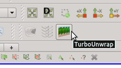
Step 2 — First, the blades need to be transformed from the cylinder- or disk-like arrangement to a straight rectangular block. This is done by the filter Turbo Unwrap. You should see the icon of the filter in the toolbar. Note that the filter is available (i.e. coloured and clickable) only when the data selected in “Pipeline browser” are of the type “Multi-block Dataset” (see panel “Information”, section “Statistics”).

27

Either use this button, or select the filter Turbo Unwrap in the Filters > Turbomachinery (or Filters > Alphabetical) menu, or use the search box from Filters > Search. This will add the filter into the “Pipeline browser”.

Step 3 — The basic properties of the filter Turbo Unwrap are shown in the figure [*]. When the advanced options are hidden, there are only a few options to define. First of all, it is necessary to choose the blade wall patch, that will be transformed, and the hub and shroud patches, which will serve as a leaders to define the transformation. After the transformation is done, hub and shroud will be perfectly flat and parallel to each other, conformly deforming the mesh in between. If multiple mesh parts are selected in the “Unwrap mesh” window or multiple patches are selected in “Hub” or “Shroud” windows then they will be internally merged into a single entity before proceeding. In this example the mesh is well prepared and we can just select the three items that we loaded in the first step.
Step 4 — Set the direction and position of the rotating axis using the parameters “Axis” and “Origin”. In our case we use $ z$-axis, which is the default option.

Step 5 — Unlike in the case of the blade-to-blade view , when constructing the pressure profile it is mostly not necessary to specify a non-zero “Clip out radius”, because the blades do not reach all the way to the axis in the middle. We will leave the parameter having its default zero value.

Step 6 — Click on “Apply”. The transformation should be relatively fast, because the sufrace mesh of the blades is orders of magnitude easier to process than the full volume mesh. It may be necessary to zoom in or out a little (depending on the geometry) to make the result fit to window. Outcome of this step is shown in the figure [*], where the blades are coloured by pressure.
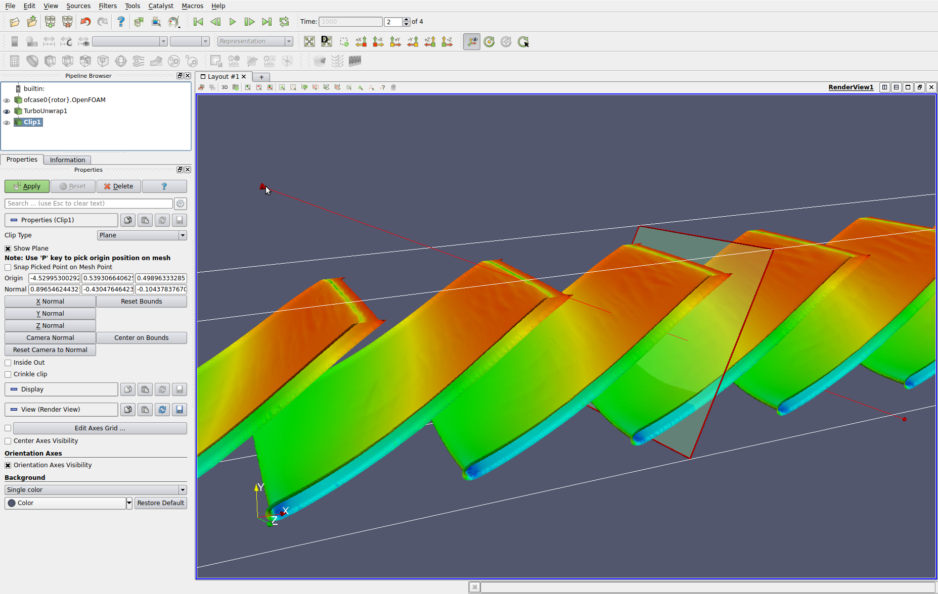
Step 7 — Having the blades transformed we can now separate the chosen blade from the rest. This is done by the filter Clip. Adding the Clip filter will provide the user with an interactive positioning tool consisting of a ball in the origin, clipping plane and its normal. Use the ball to position the plane. Use the axis to orient the plane; see figure [*]. Once you have placed the clipping plane to one side of the chosen blade so that it doesn’t intersect any blade, click apply.
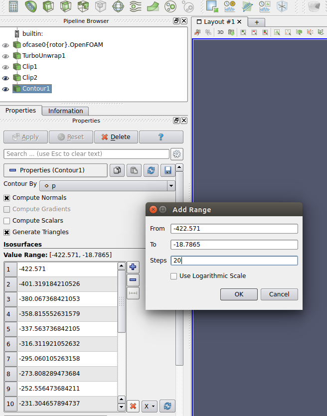
Step 9 — Append the filter Contour. In the drop-down list “Contour By” select the pressure field. Use the red cross button to erase suggested contour values (right bottom of the box “Value Range”) and then press grid button (right top) to populate the list of contour values by equidistant values covering the whole pressure range. Do not modify the suggested minimal (“From”) and maximal (“To”) values, and use e.g. 20 samples (“Steps”). See the figure [*].
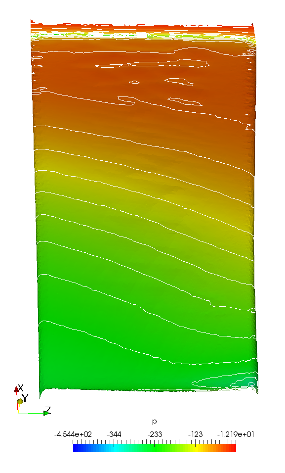
Step 10 — Pressing “Apply” will calculate the contour data and display the contours, hiding the blade geometry. Click on the eye symbol in “Pipeline Browser” to show the blade again. The results are in the figure [*].
28

Figure: Interaction with the interactive Clip manipulator when separating a single blade of a pump transformed by Turbo Blade Post / Turbo Unwrap filter. The blades are colored by static pressure calculated by TCFD using OpenFOAM.

29

Figure: Settings of the filter Contour applied on a isolated pump blade transformed by Turbo Blade Post / Turbo Unwrap filter.

30

Figure: Static pressure field and contours on an isolated blade transformed by Turbo Blade Post / Turbo Unwrap filter. The pressure data have been calculated by TCFD using OpenFOAM. Left is the pressure side, right the suction side of the blade.