Previous: Example: Blade pressure and Up: Example: Blade pressure and Next: Meridional Average filter –
This is an automatically generated documentation by LaTeX2HTML utility. In case of any issue, please, contact us at info@cfdsupport.com.
Step by step guide
![Node129 7 [*]](https://www.cfdsupport.com/wp-content/uploads/2022/02/crossref.png) .
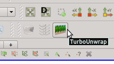
. Step 2 — First, the blades need to be transformed from the cylinder- or disk-like arrangement to a straight rectangular block. This is done by the filter Turbo Unwrap. You should see the icon of the filter in the toolbar. Note that the filter is available (i.e. coloured and clickable) only when the data selected in “Pipeline browser” are of the type “Multi-block Dataset” (see panel “Information”, section “Statistics”).
![Node129 7 [*]](https://www.cfdsupport.com/wp-content/uploads/2022/02/crossref.png) . When the advanced options are hidden, there are only a few options to define. First of all, it is necessary to choose the blade wall patch, that will be transformed, and the hub and shroud patches, which will serve as a leaders to define the transformation. After the transformation is done, hub and shroud will be perfectly flat and parallel to each other, conformly deforming the mesh in between. If multiple mesh parts are selected in the “Unwrap mesh” window or multiple patches are selected in “Hub” or “Shroud” windows then they will be internally merged into a single entity before proceeding. In this example the mesh is well prepared and we can just select the three items that we loaded in the first step.
. When the advanced options are hidden, there are only a few options to define. First of all, it is necessary to choose the blade wall patch, that will be transformed, and the hub and shroud patches, which will serve as a leaders to define the transformation. After the transformation is done, hub and shroud will be perfectly flat and parallel to each other, conformly deforming the mesh in between. If multiple mesh parts are selected in the “Unwrap mesh” window or multiple patches are selected in “Hub” or “Shroud” windows then they will be internally merged into a single entity before proceeding. In this example the mesh is well prepared and we can just select the three items that we loaded in the first step. ![Node129 7 [*]](https://www.cfdsupport.com/wp-content/uploads/2022/02/crossref.png) , where the blades are coloured by pressure.
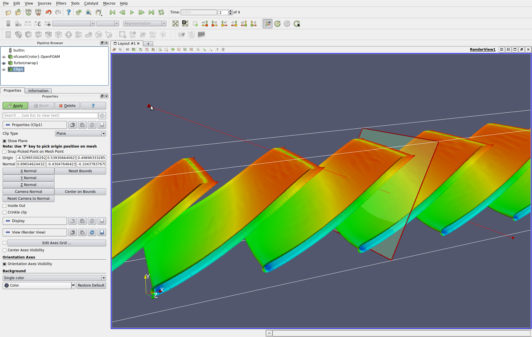
, where the blades are coloured by pressure. ![Node129 7 [*]](https://www.cfdsupport.com/wp-content/uploads/2022/02/crossref.png) . Once you have placed the clipping plane to one side of the chosen blade so that it doesn’t intersect any blade, click apply.
. Once you have placed the clipping plane to one side of the chosen blade so that it doesn’t intersect any blade, click apply. ![Node129 7 [*]](https://www.cfdsupport.com/wp-content/uploads/2022/02/crossref.png) .
. 
Figure: Interaction with the interactive Clip manipulator when separating a single blade of a pump transformed by Turbo Blade Post / Turbo Unwrap filter. The blades are colored by static pressure calculated by TCFD using OpenFOAM.

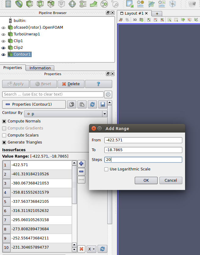
Figure: Settings of the filter Contour applied on a isolated pump blade transformed by Turbo Blade Post / Turbo Unwrap filter.

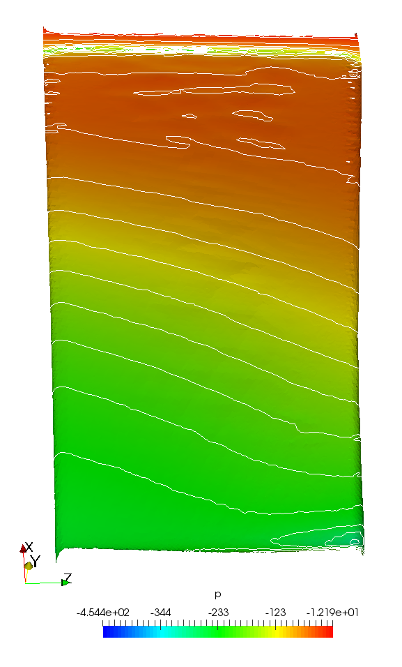
Figure: Static pressure field and contours on an isolated blade transformed by Turbo Blade Post / Turbo Unwrap filter. The pressure data have been calculated by TCFD using OpenFOAM. Left is the pressure side, right the suction side of the blade.


