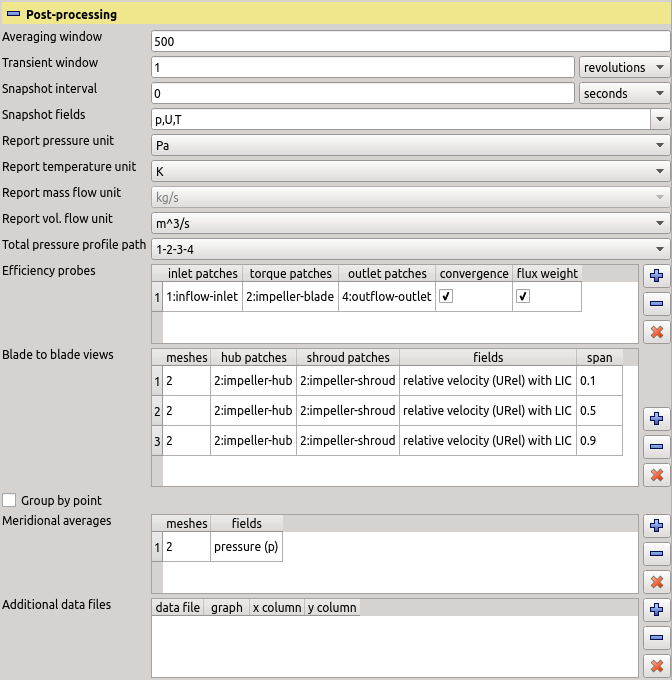
1

Previous: Running blockMesh Up: Test case: Cavity Next: Boundary and initial condition

This is an automatically generated documentation by LaTeX2HTML utility. In case of any issue, please, contact us at info@cfdsupport.com.

Test case setup

Francis Turbine Tutorial Meridional Average, ParaView window

mavg pressure 1

Figure: Turbo Blade Post; Francis Turbine Tutorial; Meridional (Circumferential) average of static pressure; OpenFOAM Water Turbine CFD

Arbitrary Mesh Interface (cyclicAMI) Boundary Condition

NOTE: cyclicAMI boundary condition is supported by boundary type cyclicAMI, defined in the mesh file boundary:


 boundaryField
 {
    rotor_periodic_1 
    {
        type            cyclicAMI;
        inGroups        1(cyclicAMI);
        matchTolerance  0.1;
        transform       rotational;
        neighbourPatch  rotor_periodic_2;
        rotationAxis    (0 0 1);
        rotationCentre  (0 0 0);
        nFaces          1628;
        startFace       171370;
    }
 }

Parameter rotationAxis defines the axis in Cartesian coordinates (directional vector of the axis).

Parameter rotationCentre is any point from the axis. So, the axis is defined by its directional vector and one of its points.
cyclicAMI boundary condition is the same for all quantities (scalars, vectors, tensors):

p, U, k, omega, epsilon, T:

 boundaryField
 {
    rotor_periodic_1 
    {
          type         cyclicAMI;
    }
 }

Previous: Simulation controls Up: TCFD – GUI Setup Next: Meshing options: Snappy hex
This is an automatically generated documentation by LaTeX2HTML utility. In case of any issue, please, contact us at info@cfdsupport.com.

Post-processing

This section allows user to define how the post-processing (evaluation of results and generation of a report) will be done.
  • The entry “Averaging window” sets the number of iterations used for calculation of the averaged fields. Also, this interval is used to monitor convergence: If the efficiency, inflow and outflow change negligibly during the window, the point is deemed converged. Finally, it acts as a smoothing interval for Figures in the resulting report.
  • The entry “Transient window” is an analogue of “Averaging window” in a transient calculation. It can be given either in seconds, or in revolutions.
  • The entry “Snapshot interval” has only effect in a transient calculation. It serves for regular write-out of the results during the calculation, so that they can be later used e.g. to construct an animation.
  • The element “Snapshot fields” can be used to select fields that will be written during a snapshot. Quantities other than velocity and pressure are rarely needed.
  • The selection “Report sections” defines sections to appear in the calculation report.
  • The selection “Report quantity” defines the reference quantity for the calculation report.
  • The selection “Report pressure unit” defines the pressure unit that will be used in the calculation report.
  • The selection “Report temperature unit” defines the temperature unit that will be used in the calculation report.
  • The selection “Report mass flow unit” defines the mass flow unit that will be used in the calculation report.
  • The selection “Report vol. flow unit” defines the volumetric flow unit that will be used in the calculation report.
  • The list “Stream path” offers the possibility to select a path though the simulated machine (in terms of component indices) that will be used when plotting the total pressure along the flow (one point per interface encountered on the way). For linear component topology with single inlet to the first component and single outlet from the last component there will be only one path and the resulting total pressure graph will simply correspond to the total pressure variations between the inlet and the outlet. But for more complicated topologies with cycles of multiple inlets/outlets there are generally more ways how to choose the path.
  • The table “Efficiency probes” has by default a single generic row, which corresponds to the default report being generated. Every row of the table defines inlet, torque and outlet patches. It is possible to add more rows to this table with different contents, so that more reports will be generated for the chosen evaluation method. The inlet and outlet patches are used to calculate mass flow and total pressure difference, the torque patches are used to calculate the torque expended by the fluid/blade (depending on the machine). Together, they are used to evaluate efficiency and other quantities. The switch “convergence” determines whether this particular probe is considered by the convergence check; the calculation will be stopped as converged only when all probes with enabled “convergence” switch sufficiently converge. The switch “flux weight” determines whether the quantities used to calculate efficiency are calculated from area-averaged or mass-flow-averaged quantities.
  • The table “Forces” contains a list of requested boundary parts on which forces and force coefficients are evaluated:
  • patches defines boundary parts for evaluation
    liftX,*Y,*Z lift direction ($ \vec L$) for the lift coefficient evaluation ($ C_l$)
    dragX,*Y,*Z drag direction ($ \vec D$) for the drag coefficient evaluation ($ C_d$)
    pitchX,*Y,*Z pitch axis ($ \vec P$) for the momentum coefficient evaluation ($ C_m$)
    torqueX,*Y,*Z custom axis for torque evaluation (T_axis column in output file)
    ref. area reference area ( $ A_\mathrm{ref}$) for lift and drag coefficient evaluation
    ref. length reference length ( $ l_\mathrm{ref}$) for momentum coefficient evaluation
    ref. Umag reference velocity ( $ \vert U_\mathrm{ref}\vert$) for force coefficient evaluation
    The force coefficients are evaluated as follows:
    \begin{displaymath}\begin{split}C_l &= \frac{\vec F_t\cdot \vec L}{\frac{1}{2}\rho_\mathrm{ref}\vert U_\mathrm{ref}\vert^2A_\mathrm{ref}} \\ C_d &= \frac{\vec F_t\cdot \vec D}{\frac{1}{2}\rho_\mathrm{ref}\vert U_\mathrm{ref}\vert^2A_\mathrm{ref}} \\ C_m &= \frac{\vec M_t\cdot \vec P}{\frac{1}{2}\rho_\mathrm{ref}\vert U_\mathrm{ref}\vert^2l_\mathrm{ref}A_\mathrm{ref}}\,, \end{split}\end{displaymath} (4.1)
      where $ \vec F_t$ denotes the total force and $ \vec M_t$ the total moment. For incompressible simulation the reference pressure $ \rho_\textrm{ref}$ is taken from the value defined in Physics menu, see Page [*]. Besides the values described above, the output additionally includes force components in x,y,z direction as well as torque components for x,y,z axes.
  • The table “Blade to blade views” contains a list of requested blade-to-blade views (circularly unwrapped and slices meshes) to be generated by Turbo Blade Post. The column “meshes” contains a list of meshes that will be unwrapped. It is possible to use both the internal meshes and individual patches. The hub and shroud patches must be provided in the next two columns as they define the requested transformation of the mesh. The column “fields” is used to select the field that will be displayed on the blade-to-blade view. Finally, “span” contains a space-separated list of positions between the hub and the shroud where the blade-to-blade views will be taken.
  • The switch “Group by point” reorders the blade-to-blade views in the report so that figures corresponding to the same calculation point are grouped together; otherwise figures corresponding to the same span are grouped together. The former option is good for visualisation of how the field changes in space, whereas the latter option is good for visualisation of how the field changes with the boundary condition.
  • The table “Meridional averages” contains a list of meridional averages to be generated by Turbo Blade Post. It can be used only with component indices, but otherwise the meaning of its columns is identical to “Blade to blade views”.
  • The table “Additional data files” is used to add user data to the graphs in the final report from the calculation. The data should be provided in the form of Gnuplot-readable data files, i.e. text files with white-space-separated equal-length columns of numbers. The graph into which the data are to be added is chosen in the second column, the column indices to be used in the remaining two (first column has index 1). Several data-lines within a single data file can be achieved by interrupting the columns by an empty row; this is useful particularly in the multi-speedline summary diagrams (their name ends with “-all”).
cfd processor TCFDSource post processing

Figure: Plugin TCFDSource – post-processing.