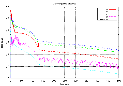


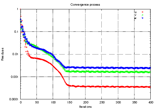
 One can continually watch the convergence of velocity vector components during the computation using a small script for gnuplot that is given in the following listing. Let’s name the file residual.gp.
# Gnuplot script file for plotting data from file "log" set title "Convergence process" set xlabel "Iterations" set ylabel "Residuals" set grid set logscale y plot "< cat log | grep Ux | cut -d' ' -f9 | tr -d ','" title 'u', \ "< cat log | grep Uy | cut -d' ' -f9 | tr -d ','" title 'v', \ "< cat log | grep Uz | cut -d' ' -f9 | tr -d ','" title 'w' pause 10 # or "pause mouse" reread- The script expects the output of the solver to be in the file log. If any other output file is to be used, e.g. log.simpleFoam , one has first to create a symbolic link named log.
# ln -s log.simpleFoam log
# gnuplot residual.gp
- One can reconstruct the case after the end of parallel computation by running command:
# reconstructPar -latestTime - The switch -latestTime tells the utility reconstructPar to reconstruct just the last time level, because the case is computed as a steady state simulation.
- The results can be analyzed using paraview. Either simply run paraFoam without any arguments as usually, or create first carNoMotor.OpenFOAM placeholder file by typing
# paraFoam -touch
and then run ParaView without the OpenFOAM wrapper paraFoam:
# paraview - To load the case results into plain ParaView select File
 Open and open the placeholder *.OpenFOAM file.
 - ParaView uses “states”, which are prepared templates for visualization of the cases. They contain an already populated pipeline and view transformations.
- A prepared scene can be saved as a ParaView state using the menu item File Save state.
- NOTE: ParaView state file *.pvsm provides absolute path to the *.OpenFOAM placeholder.
- To load a preset “state” into ParaView delete all objects from the pipeline and select File Load State and choose a prepared template, e.g. pvsm/uField.pvsm.
- NOTE: The absolute path to the *.OpenFOAM placeholder in loaded “state” file may differ from current path to the *.OpenFOAM placeholder. If the path is different ParaView ask you for it via “Fix Paths in State File” window.
- The template uField displays velocity field in xy plane and stream lines around a car body.
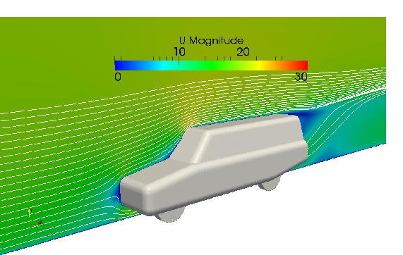
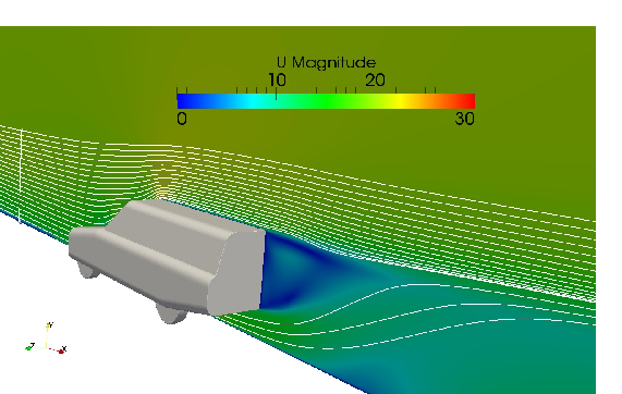
Figure: OpenFOAM tutorial car case. Velocity field in the ![]() plane and stream lines
plane and stream lines
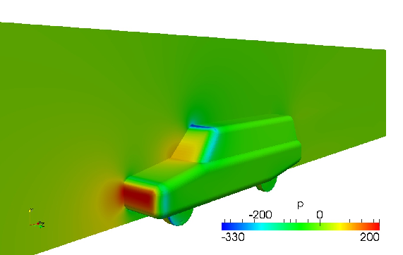
Figure: OpenFOAM tutorial car case. Pressure field in the ![]() plane and pressure distribution on the car body
plane and pressure distribution on the car body
- Similarly, loading the template pField.pvsm will display the pressure field in the
 plane and the pressure distribution on a the car body.
 - The utility foamLog
 log
log  can be used to extract all interesting data from log file.
 - All the data obtained by foamLog can be visualized using gnuplot.
- The reader can find more information about foamLog log in the chapter “Backward-facing step” of CFD support manual part I.
- A sample script allresiduals.gp is in the case directory.