Axial Fan Simulation-Driven Optimization
This study shows a CFD-driven optimization workflow of an axial fan using a simulation environment TCAE

Axial Fan Optimization - Introduction
Axial fans are widely used in various industries such as ventilation, cooling, heating, and aerospace. Axial fans are devices that move air or gas parallel to the axis of rotation of the blades. They have many advantages such as high efficiency, low noise, and easy installation. However, they also face some challenges such as blade erosion, vibration, and flow separation. Therefore, many researchers have tried to optimize the design and performance of axial fans using various methods such as simulation, experimentation, and machine learning. In this case study, we will show the recent developments and applications of simulation-driven optimization for axial fan design using the simulation environment TCAE.

CFD simulation-driven optimization of axial fans is a novel and effective method to improve the performance and efficiency of axial fans, which are widely used in various fields such as ventilation, cooling, and propulsion. By using numerical aerodynamic and structural analysis tools, and optimization algorithms, the optimal design parameters of the axial fan blades can be obtained under different operating conditions and constraints. The optimization process involves parametrizing the blade geometry, performing CFD simulations, evaluating the objective function and constraints, and updating the design variables until convergence.

This particular case study deals with the parametric optimization of an axial fan. The field of shape optimization is extremely broad and it’s impossible to cover a complex optimization of all possible parameters whatsoever. In this case study, we have chosen a couple of parameters that show the potential of using methods that create a consistent engineering workflow.

Axial Fan Parametric Model - Geometry Description
The axial fan in this study is a relatively standard piece of turbomachinery based on the experiments and measurements and the details can be found in the references [1], [2], [3].
In the simulation model, the complexity of the actual fan system is simplified. It is represented as a fan that generates airflow between two chambers or rooms.

The axial fan under investigation in this study exhibits specific geometric dimensions. The blade tip diameter measures 500 mm, providing an indication of the fan’s overall size. The chambers, on the other hand, possess widths and heights of 2400 mm, accommodating the flow generated by the fan. The complete model, comprising the fan and the chambers, has a length of 3376 mm, capturing the extent of the entire setup.
To facilitate the design process and enable parametric variations, a parametric model of the axial fan was developed using OpenVSP. OpenVSP serves as a versatile software tool that offers automated parametric geometry generation. By employing OpenVSP, researchers can efficiently construct the initial design of the axial fan and subsequently explore a wide range of design parameters.
Furthermore, OpenVSP’s capabilities extend beyond the initial design phase. It is also employed within the optimization loop, where it plays a crucial role in automated parametric geometry manipulation.

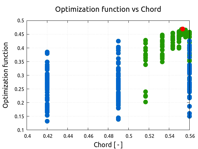
When designing such a parametric model, the task is extremely complex and there are infinite degrees of freedom in terms of parameters. For the purposes of this study, the authors have chosen four parameters to be variable and the rest of the parameters are kept constant. The variable parameters are the number of blades, blade chord length, blade thickness, and blade twist angle. The chord parameter is a bounded ratio of the airfoil profile chord (NACA 4510 Airfoil M=4.0% P=50.0% T=10.0%) and the blade length.
| Variable Parameter | min | max |
|---|---|---|
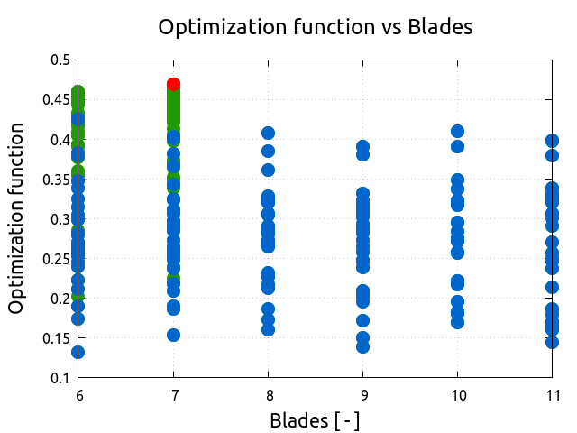
| number of blades [-] | 6 | 11 |
| chord [-] | 0.42 | 0.56 |
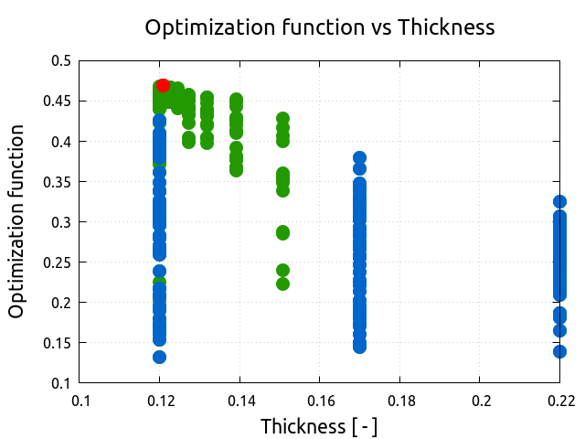
| thickness [m] | 0.12 | 0.22 |
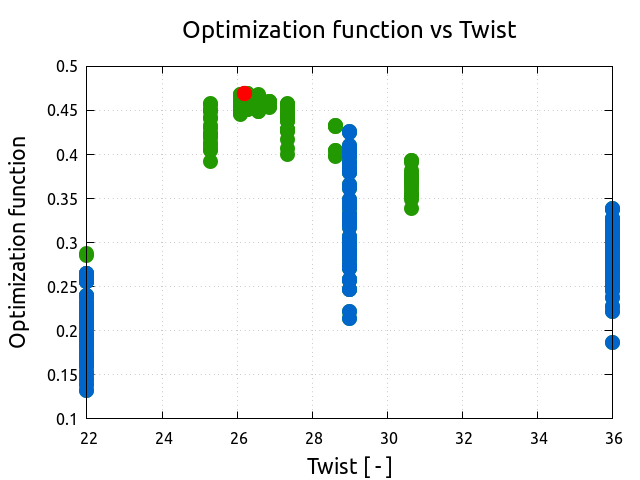
| twist [degrees] | 22 | 36 |
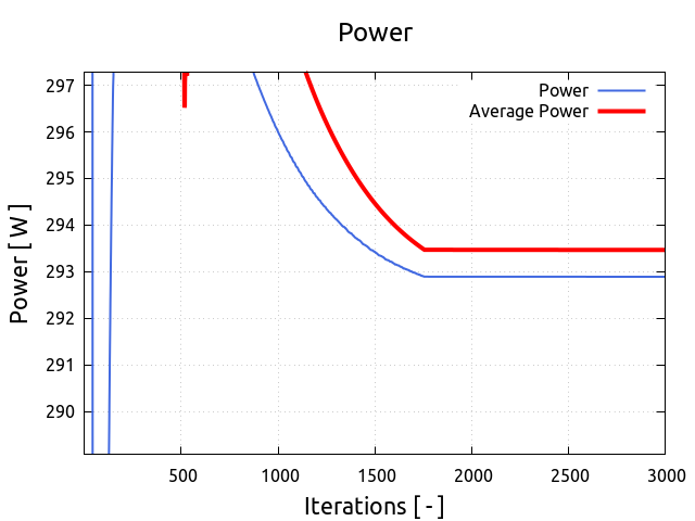
Fan efficiency has been chosen as an optimization function. Additionally, fan power and generated pressure difference have been chosen as secondary followed quantities.
Axial Fan - CFD Simulation Preprocessing
A typical input for a detailed simulation analysis is a 3D surface model in the form of an STL surface, together with related physics and boundary conditions. For CFD simulation, it is needed to have a simulation-ready surface, which is a closed watertight model (sometimes also called waterproof, model negative, or wet surface) of the model’s parts where the fluid flows. The simulation domain consists of two chambers divided by a wall. The axial fan blows the air from one room to the other.

For CFD simulation it is best to split the geometry into several waterproof components because of rotation (some parts may be rotating and others not). Each component itself has to be waterproof and consists of a few or multiple STL surfaces. It is smart to split each component into multiple surfaces (more is better) because it opens a broader range of meshing options, simulation methods (mesh refinements, manipulation, boundary conditions, evaluation of results on model-specific parts, …), and postprocessing.

The principle is always the same: the 3D surface model has to be created; all the tiny, irrelevant, and problematic model parts must be removed, and all the holes must be sealed up (a watertight surface model is required).
This axial fan CAD model is relatively simple. The final surface model in the STL format is created as input for the meshing phase. This preprocessing phase of the workflow is extremely important because it determines the simulation potential and limits the CFD results.

In this axial fan optimization project, the OpenVSP model has been split into three logical parts:
- Inlet room
- Rotor
- Outlet room
In the CFD methodology employed for this study, the surface model data, representing the geometry, is stored in .stl file format. Along with the geometric information, the necessary physical inputs, such as boundary conditions and material properties, are also loaded into the TCFD software.
In addition to the .stl file format, there are alternative options available for mesh loading in TCFD. Users have the flexibility to import an external mesh in OpenFOAM mesh format, which offers compatibility with other simulation tools within the OpenFOAM framework. Alternatively, TCFD supports loading meshes in MSH format (Fluent mesh format) or CGNS mesh format, providing a wider range of mesh compatibility options.
TCFD module follows a multi-component approach. This means that the model is divided into several distinct components or regions, each serving a specific purpose or containing specific properties. In TCFD, each region can have its own dedicated mesh, allowing for finer control over the discretization and resolution of different regions within the model.
This CFD methodology employs a multi-component approach, which means the model is split into a certain number of components. In TCFD each region can have its own mesh and individual meshes communicate via interfaces.

IMPORTANT NOTICE ON PREPROCESSING
The surface of the simulation-ready model has to be clean. The principle is always the same: the watertight surface model has to be created; all the tiny, irrelevant, and problematic model parts must be removed, and all the holes must be sealed up (the watertight surface model is required). The preprocessing phase is an extremely important part of each simulation workflow. It sets up all the simulation potential and limitations. It should never be underestimated. Mistakes or poor quality engineering in the preprocessing phase can be hardly compensated later in the simulation phase and post-processing phase. For more details, see the TCAE documentation.
Axial Fan - CFD Meshing
The computational mesh for CFD is created using the snappyHexMesh open-source application within an automated software module called TMESH. All the mesh settings are configured in the TCAE GUI.

Every project simulated in TCFD has its component graph. The component graph is a simple scheme that shows how the components are organized. The flow model topology, the inlet, the outlet, and how the components are connected via interfaces.

For each model component, a cartesian block mesh is created (box around the model), as an initial background mesh, that is further refined along with the simulated object. The basic mesh cell size is a cube defined with the keyword “background mesh size“. The mesh is gradually refined to the model wall. The mesh refinement levels can be easily changed, to obtain the coarser or finer mesh, to better handle the mesh size. Inflation layers can be easily handled if needed. As already stated, one of the key things to perform a good CAA simulation is a choice of a representative control surface. Its properties were described in the previous section. The generation of the control surface is executed in GMSH meshing software with desired shape and accuracy specified.

The total number of mesh cells is always a big question for every CFD project. In this particular case, we run several meshes with the various number of mesh cells, varying from 2 million to 12 million with no major effect on the results. However, the proper mesh (grid) dependence study should be done. The exact mesh settings remain the object of future investigation.
Axial Fan - CFD Simulation Setup
The CFD simulation in this project is facilitated through the utilization of the TCAE software module TCFD. The entire setup and execution of the CFD simulation are performed within the TCFD GUI integrated with ParaView. TCFD, being based on the OpenFOAM open-source software, provides a powerful foundation for accurate computational fluid dynamics simulations.
The simulation setup process involves navigating through the GUI from the top menu to the bottom, allowing for a systematic configuration of various parameters and settings. This GUI-driven approach ensures a user-friendly experience and enables researchers to define the simulation environment in a step-by-step manner, tailoring it to the specific requirements of the study. By leveraging the intuitive interface, researchers can efficiently set up their simulation, defining boundary conditions, solver options, mesh properties, and other relevant aspects, leading to a comprehensive and accurate CFD simulation.

- Simulation type: Fan
- Time management: steady-state
- Physical model: Incompressible
- Number of components: 3 [-]
- Wall roughness: none
- Speed: 1486 [RPM]
- Outlet: Static pressure 0 [m2/s2]
- Turbulence: RANS
- Turbulence model: k-omega SST
- Shear Thinnig model: Newtonian
- Wall treatment: Wall functions
- Turbulence intensity: 5%
- Speedlines: 1 [-]
- Simulation points: 1 [-]
- Fluid: Air
- Reference pressure: 1 [atm]
- Dynamic viscosity: 1.8 × 10E-5 [Pa⋅s]
- Reference density: 1.2 [kg/m3]
- CFD CPU Time: 7.5 core.hours/point
- BladeToBlade: off
Axial Fan - Optimization Setup
The optimization loop is managed with the software module TOPT. Complete optimization setup and run are done in the TCAE GUI.

The optimization loop is a set of individual simulation runs in a sequence. In the beginning, the sequence of pre-set simulations (DOE – design of experiment) is run. After that, the optimization part is executed. The optimization algorithm suggests a set of parameters and the simulation is executed. After each run, the results (Optimization function = Objective function) are evaluated and the optimization algorithm designs a new set of parameters. The optimization flow chart is the following:
Optimization Settings
- Operation mode: optimize
- Algorithm: golden section search
- Max runs: 400
- Number of parameters: 4
- Number of DOE runs: 6x3x3x3
- Optimization function: efficiency
- Followed quantity: power
- Followed quantity: pressure

Simulation Loop Run

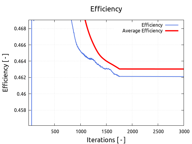
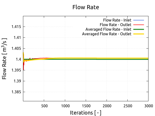
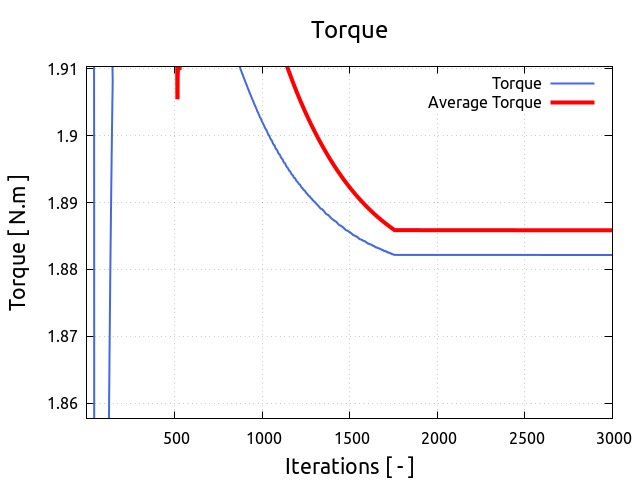
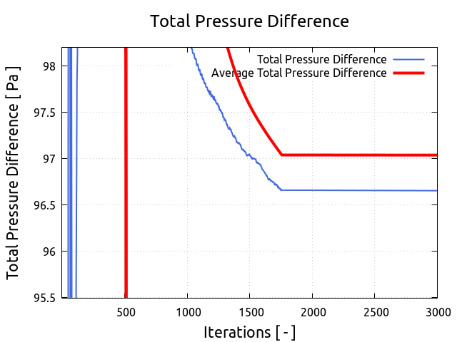
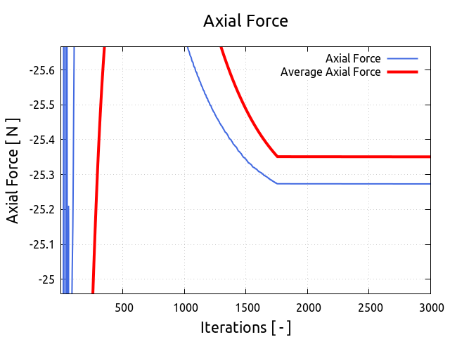
TCFD includes a built-in post-processing module that automatically evaluates all the required quantities, such as efficiency, torque, forces, force coefficients, flow rates, pressure, velocity, and much more. All these quantities are evaluated throughout the simulation run, and all the important data is summarized in an HTML report, which can be updated anytime during the simulation, for every run.
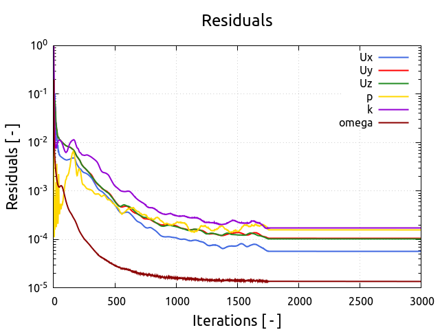
All the simulation data are also saved in tabulated CSV files for further evaluation. TCFD is capable of writing the results down at any time during the simulation. The convergence of basic quantities and integral quantities is monitored still during the simulation run. The geometry was created one time using TCAD in the preprocessing phase. First, the TMESH is executed to create the volume mesh for CFD. Then the CFD simulation is executed and evaluated. TOPT module creates the new set of data and the simulation loop continues with the new simulation run.
Axial Fan - Post-processing - Integral Results
The integral results and simulation statistics are evaluated automatically for every simulation run. Every simulation run in TCAE has its own unique simulation report. The integral results both for CFD and FEA are written down in the corresponding HTML or PDF reports.

All the relevant integral quantities are evaluated, sorted, and stored in the corresponding CSV files and are ready for further usage. The following integral quantities are evaluated every time step.
The integral results and simulation statistics are evaluated automatically for every simulation run. Every simulation run in TCAE has its own unique simulation report. The integral results both for CFD and FEA are written down in the corresponding HTML or PDF reports.
All the relevant integral quantities are evaluated, sorted, and stored in the corresponding CSV files and are ready for further usage. Following integral quantities are evaluated every time step.

FDA Pump - Postprocessing - Volume Fields
Once the simulation is completed, the integral results obtained from the CFD analysis are stored in CSV files, making them easily accessible for further post-processing and analysis. These results capture important information such as forces, pressures, velocities, and other relevant variables.

To perform a more detailed visualization and analysis of the volume fields, researchers turn to ParaView, an open-source visualization tool widely used in the CFD community. ParaView offers a comprehensive suite of tools and methods specifically designed for CFD post-processing and result evaluation.

Within ParaView, users can leverage numerous filters and sources to enhance their understanding of the simulated flow. These filters and sources include a range of powerful tools, such as the Calculator, Contour, Clip, Slice, Threshold, Glyph (Vectors), and Streamtraces (Streamlines), among others. Each of these tools serves a specific purpose and allows for the extraction of valuable insights from the simulation data.

Furthermore, ParaView supports various visualization techniques like glyphs, streamlines, and streamline seeding for visualizing vector fields, providing a comprehensive view of the flow patterns and directions.

By utilizing ParaView’s extensive range of filters and sources, researchers can effectively extract and visualize key features and phenomena from the CFD simulation results, gaining deeper insights into the underlying physics and flow behavior.

The combination of CSV files for integral results and ParaView for volume field post-processing empowers users to perform a thorough analysis of the CFD data, facilitating comprehensive understanding and effective decision-making.

All the images can be created manually or scripted because ParaView can run without opening the ParaView GUI, which is controlled through Python. There are two Python interfaces – PvPython and PvBatch.
Optimization Results
In the TCAE optimization process an automated generation of a TOPT report is carried out. This report serves as a comprehensive summary, encompassing crucial information regarding the optimization procedure and its outcomes.
The TOPT report includes various key elements that aid in understanding and analyzing the optimization process. First and foremost, it provides essential simulation statistics, offering insights into the computational aspects of the optimization. These statistics encompass metrics such as setup information, computational time, and resource utilization.
Furthermore, the TOPT report presents a detailed list of the simulated points from the parametric space. This list provides a record of the different parameter combinations that were evaluated during the optimization. Researchers can refer to this list to track the progression of the optimization and understand the specific parameter settings explored throughout the process.
To facilitate visualization and interpretation, the TOPT report includes 2D and 3D plots that encapsulate important aspects of the optimization results.

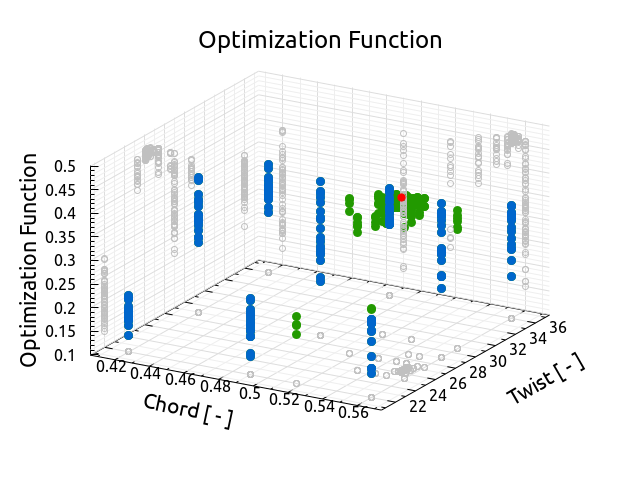
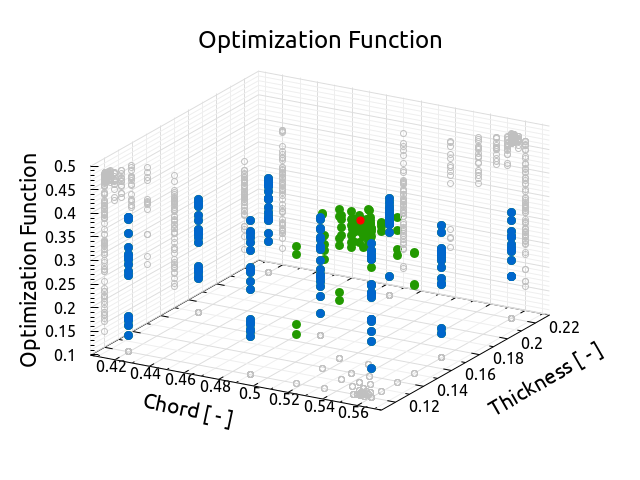
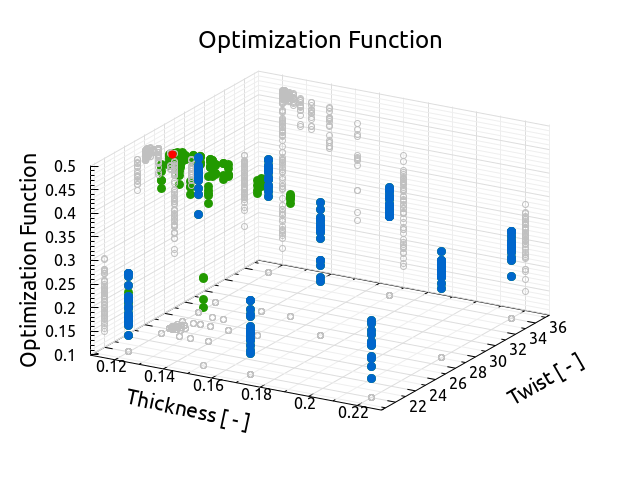
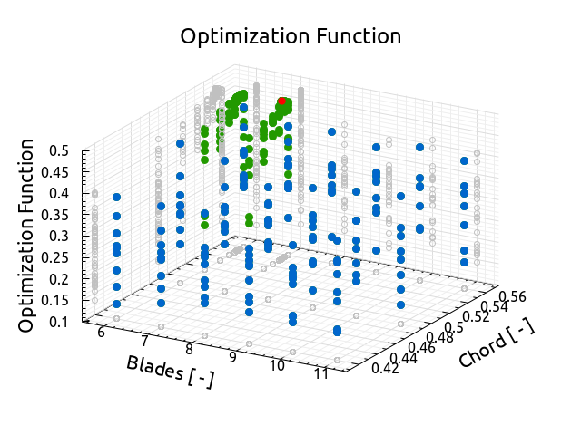
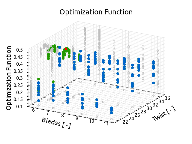
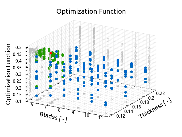
The principal quantity followed is the optimization (object) function because the whole optimization loop is based on it. It’s important to see how it develops over simulation runs. In this case, the objective function is the fan efficiency and the goal is to maximize it.

The blue color simulation points show the DOE phase. The green color points show the optimization phase. The red point signs the maximum of the objective function which was achieved in run #370 (46.88%).
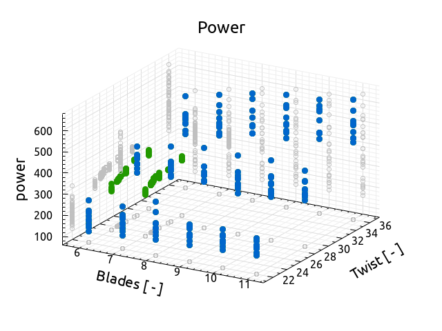
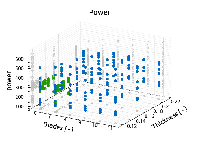
Additional important quantities to be followed are power and total pressure difference.

A very useful type of optimization data visualization is a 2D plot of the Optimization (objective)
function vs individual variable parameters. It’s important to make sure that the “winning” simulation points are not stuck to the min or max values of each variable parameter.
Similar sensitivity plots can be visualized in semi-3D plots which show the optimization function or any other tracked quantity as a function of two variables. The following plots show some combinations of parameters.

Conclusion
- It has been shown how to make a CFD-simulation-driven optimization of the real-world axial fan in a single automated workflow.
- This study clearly shows the importance of the optimization process. The fan performance is extremely non-intuitive. The following set of images shows four very similar axial fans of this optimization loop. There are very small differences in details among them (difficult to recognize by the human eye) but fans’ performances differ drastically. There are four very similar fans and their efficiencies are 36%, 40%, 43%, and 47%.


- The simulation loop of 400 individual CFD runs has taken 121 hours on 24 cores.
- The optimization project is an extremely complex task and there is always a lot of space for improvements. This study is rather an example to show the optimization possibilities.
- TCAE showed to be a very effective tool for CFD and optimization for all rotating machinery in general.
- This study was intentionally written in short not to overwhelm its readers with too many details. The original intention was to show the modern simulation workflow and its potential.
- The original fan & measurement details are listed in the references below.
- All the technical details regarding CFD & optimization are listed in the TCAE manual.
- Complete simulation reports can be found on the CFDSUPPORT website https://www.cfdsupport.com/axial-fan-simulation-driven-optimization.html
- The whole workflow is anytime repeatable, the case geometry and data are freely available for download on the CFDSUPPORT website.
- More information about TCAE can be found on the CFD SUPPORT website: https://www.cfdsupport.com/tcae.html
- Questions will be happily answered via email info@cfdsupport.com
References
[1] Manfred Kaltenbacher, Stefan Schoder. EAA Benchmark for an axial fan. e-Forum Acusticum 2020,
Dec 2020, Lyon, France. pp.1333-1335, 10.48465/fa.2020.0194. hal-03221387
[2] Stefan Schoder, Clemens Junger, Manfred Kaltenbacher. Computational aeroacoustics of the EAA benchmark case of an axial fan, Acta Acust. 4 (5) 22 (2020), DOI: 10.1051/aacus/2020021
[3] Krömer, Florian. (2018). Sound emission of low-pressure axial fans under distorted inflow conditions. 10.25593/978-3-96147-089-1.
[4] TCAE Training – https://www.cfdsupport.com/download-documentation.html
[5] TCAE Manual – https://www.cfdsupport.com/download-documentation.html
[6] TCAE Webinars – https://www.youtube.com/playlist?list=PLbxC_ERCZDHbytN1WvSRi57eksKTNtTis
Download TCAE Tutorial - Axial Fan Optimization
File name: axial-fan-optimization-TCAE-Tutorial.zip
File size: 30 MB
Tutorial Features: CFD, TCAE, TMESH, TCFD, TOPT, SIMULATION, AXIAL FAN, OPTIMIZATION, TURBOMACHINERY, INCOMPRESSIBLE FLOW, INCOMPRESSIBLE, RANS, BLOOD FLOW, STEADY-STATE, AUTOMATION, WORKFLOW, AXIAL FLOW, FULL IMPELLER, SNAPPYHEXMESH, 3 COMPONENTS, RPM=1486