


Visual postprocessing can be done in paraview. This case brings new problem – How to visualize Lagrangian fields?
- Run paraview in case directory, i.e. use paraFoam command.
- Load the case, make just boundary visible (check only patches in Mesh parts).
- Make few clips to see just backward walls.
- Load the case again and go to the last time step.
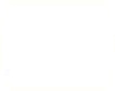
- Check kinematicCloud from Mesh Parts menu and check all Lagrangian Fields (see Fig.
 ).
).
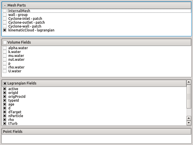
- Instead of surface representation use Point Gaussian (see Fig. ).
- The particles setup is now available in Properties menu (see Fig. ).
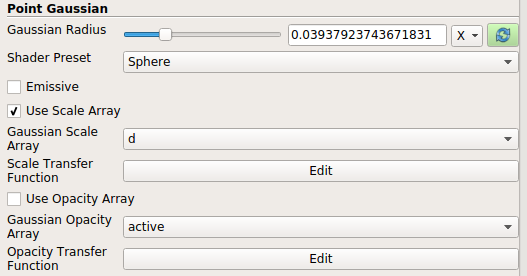
- There is several option how to visualize particels. We can visualize its diameters by checking Use Scale Array and choosing “d” in Gaussian Scale Array menu and clicking on Edit Scale Transfer Function.
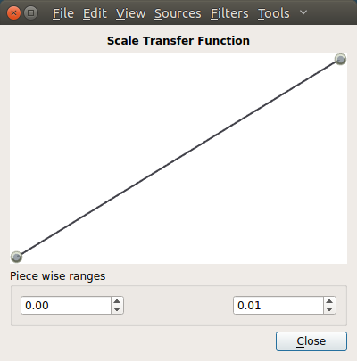
- In the Edit Transfer Function (see Fig. ) set Piece wise ranges to desired range (usualy your current data range), in our case from 0.00 to 0.01.
- For transient cases a time information is important; Go to menu Filter -> Alphabetical -> Annotate Time Filter.
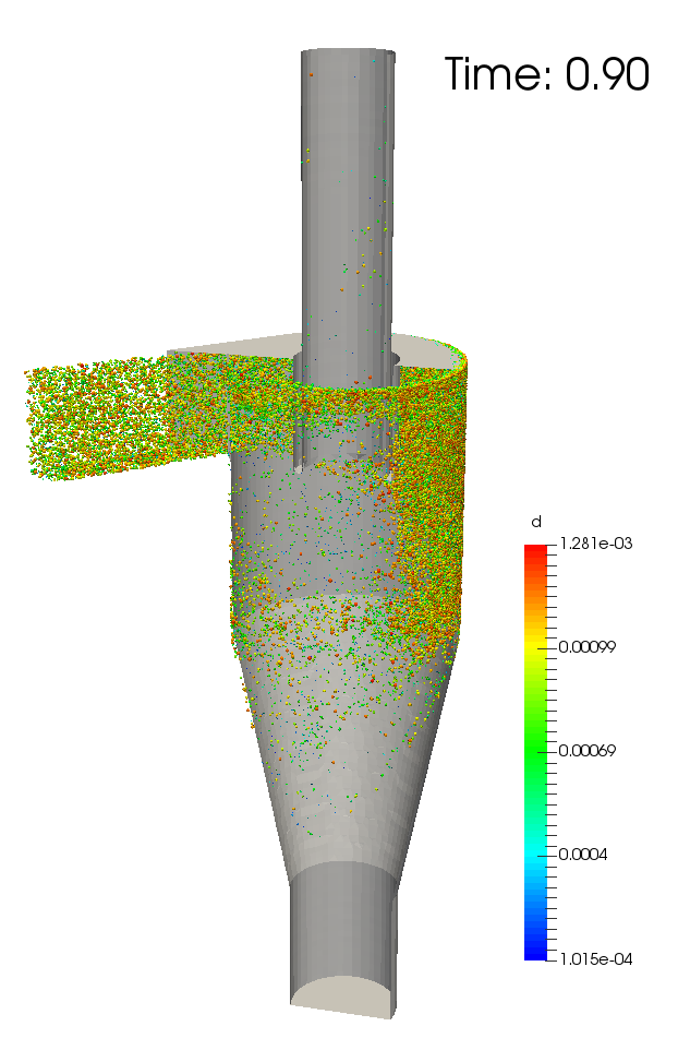
- Final view is depicted in Figure