


Spalart-Allmaras model (SA) presented by Spalart and Allmaras [11] is an one-equational model written in terms of modified eddy viscosity. The model uses empiricism and arguments of dimensional analysis, it is independent on  , but requires the distance to the nearest wall
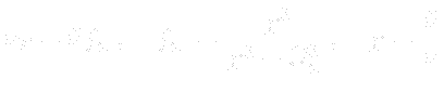
  . The turbulent eddy viscosity is developed with the help of model’s transport equation:
where the production term is developed with the help of norm of vorticity
. The turbulent eddy viscosity is developed with the help of model’s transport equation:
where the production term is developed with the help of norm of vorticity  . The diffusion terms are naturally connected with spatial derivatives of
  . The destruction term arose from dimensional analysis.
  and
and  are transition functions, that provide control over the laminar and turbulent regions. All the details are step by step discussed in the original article [11]. The turbulent eddy viscosity is then:
where 

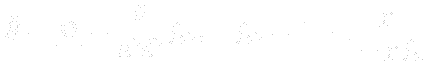
 is Reynolds turbulent number. Model is completed by following formulas:
The following table gives the model constants present in the formulas above:
Subsections
![\begin{multline} \frac{\partial \tilde{\nu}}{\partial t} + u_j \frac{\partial \tilde{\nu}}{\partial x_j} = \underbrace{ C_{b1} [1 - f_{t2}] \tilde{S} \tilde{\nu} }_{\text{production term}} + \underbrace{ \frac{1}{\sigma} \{ \frac{\partial }{\partial x_j} [(\nu + \tilde{\nu}) \frac{\partial \tilde{\nu}}{\partial x_j}] + C_{b2} \frac{\partial \tilde{\nu}}{\partial x_j} \frac{\partial \tilde{\nu}}{\partial x_j} \} }_{\text{diffusion term}} - \\ - \underbrace{ \left[C_{w1} f_w - \frac{C_{b1}}{\kappa^2} f_{t2}\right] \left( \frac{\tilde{\nu}}{d} \right)^2 }_{\text{destruction term}} + f_{t1} \Delta U^2 \end{multline}](https://www.cfdsupport.com/wp-content/uploads/2022/02/img489.png)
 |
(27.29) |
 |
(27.30) |
![$\displaystyle f_w = g \left[ \frac{ 1 + C_{w3}^6 }{ g^6 + C_{w3}^6 } \right]^{1/6}, \quad g = r + C_{w2}(r^6 - r), \quad r \equiv \frac{\tilde{\nu} }{ \tilde{S} \kappa^2 d^2 }$](https://www.cfdsupport.com/wp-content/uploads/2022/02/img498.png) |
(27.31) |
![$\displaystyle f_{t1} = C_{t1} g_t \exp\left( -C_{t2} \frac{\omega_t^2}{\Delta U^2} [ d^2 + g^2_t d^2_t] \right)$](https://www.cfdsupport.com/wp-content/uploads/2022/02/img499.png) |
(27.32) |
| (27.33) |
| 0.1355 | 0.622 | 0.41 | 0.3 | 2.0 | 7.1 | 1.0 | 2.0 | 1.1 | 2.0 |
Subsections